Quantum Systems and Their Applications

Quantum information science represents one of the most significant advancements in modern technology, offering unprecedented opportunities for revolutionary breakthroughs in computing, communications, and sensing applications [Arute et al., 2019, Deshpande et al., 2022, Wu et al., 2021, Zhong et al., 2020, Zhu et al., 2022]. This interdisciplinary field leverages the principles of quantum mechanics, exploiting phenomena such as superposition, entanglement, and quantum coherence to enhance computational capabilities and security far beyond the reach of classical systems [Silverman, 2008, Qiao et al., 2017, Xi et al., 2015]. Quantum technologies have demonstrated considerable promise in tackling computationally challenging problems across diverse domains, including cryptography, materials science, pharmaceutical development, and complex optimization problems.

At the heart of quantum information technology lies the quantum bit, also known as a qubit. Unlike classical bits that encode information strictly in binary states (0 or 1), qubits capitalize on the quantum mechanical principle of superposition, enabling simultaneous existence in multiple states [LaPierre, 2021]. This extraordinary capability allows quantum systems to accelerate computational tasks exponentially. Quantum algorithms, such as Shor’s algorithm for integer factorization and Grover’s algorithm for database searches, exemplify this superior computational power, providing significant speed-ups compared to classical algorithms [Nielsen and Chuang, 2010, Xu et al., 2021, Guo, 2023]. Additionally, quantum computing promises substantial advancements in simulating quantum mechanical systems, which will significantly benefit chemical simulations, materials discovery, and drug development [Barkoutsos et al., 2021, Vakili et al., 2024].

A new and distinct quantum state that emerges from specific quantitative relationships with initial states is known as a superposition of these original states. Beyond enabling the superposition of states, the phenomenon of entanglement, where subsystems become intricately correlated, significantly amplifies the computational prowess of qubits [Hughes et al., 2021, Montanaro, 2016]. Nevertheless, these quantum states are exceptionally fragile, with environmental interactions rapidly causing decoherence and the subsequent collapse of quantum coherence. Due to this rapid loss of coherence, it remains exceedingly challenging to reliably create and maintain initial quantum superposed states for practical applications.

Granular Systems and Their Application in Quantum Systems

Granular systems, consisting of discrete macroscopic particles interacting through strongly nonlinear contact forces, represent a compelling domain for exploring quantum-inspired phenomena within classical frameworks. These systems, composed of particles typically interacting via Hertzian contact mechanics, are uniquely positioned at the intersection of nonlinear dynamics and classical mechanics, exhibiting rich and complex behaviors such as solitary wave propagation, nonlinear resonances, and nonlinear normal modes [King and Vakakis, 1995].

Unlike traditional linear elastic media, granular systems inherently feature nonlinear interactions due to their geometry-dependent force-displacement relationships. This intrinsic nonlinearity facilitates dynamic phenomena closely analogous to quantum mechanical concepts, including the formation of stable superpositions and classical analogues of quantum entanglement [Hasan and Deymier, 2022]. Such properties make granular media especially promising as platforms for developing macroscopic quantum analogues, robust systems that can mimic quantum-like behavior at room temperature and under practical environmental conditions.

Limitations of the Quantum Mechanical System

Consequently, quantum systems used in practical quantum computing applications typically require stringent environmental conditions, such as ultra-low temperatures near absolute zero, vacuum environments, and electromagnetic shielding [Narasimhachar and Gour, 2015, Kato, 2015, Weber et al., 2022]. These extreme conditions significantly limit the practical implementation of quantum systems, thus hindering widespread adoption. Research efforts have successfully demonstrated quantum superposition experimentally in various microscopic systems, such as trapped ions, Bose-Einstein condensates, and atomic ensembles, achieving remarkable precision under carefully controlled laboratory conditions [Ruostekoski et al., 1998, Huang and Moore, 2006, Brune et al., 1996].

Recognizing the significant hurdles presented by quantum decoherence and the challenges faced by topological quantum computing, researchers have actively pursued alternative strategies involving macroscopic superpositions in classical systems. These macroscopic superposition states, which can be achieved at room temperature and in less stringent environments, present compelling avenues for robust quantum-like computation [Deymier and Runge, 2017, Calderin et al., 2019]. Recent successful demonstrations of macroscopic superposition have included experiments with trapped ions, atomic ensembles, and mechanical oscillators interacting with spin qubits, opening up possibilities for exploring quantum-like phenomena on macroscopic scales [Sánchez Muñoz et al., 2018, Wood et al., 2022].

Motivation of the Study

To overcome these limitations, researchers have explored alternative approaches, such as topological quantum computing (TPC), where the quantum information is encoded using topological properties on a macroscopic scale. TPC leverages non-Abelian statistics and topological states of matter to create more robust qubits that are inherently resistant to decoherence [Freedman et al., 2001, Alicea et al., 2011]. However, recent challenges highlighted by researchers, including a notable critique by Frolov in Nature, have cast doubt on the feasibility of reliably generating and detecting topological qubits, such as Majorana particles [Frolov, 2021]. The certainty and advancement of TPC techniques have been limited by this argument, leading to a broader search for stronger and more practical substitutes.

The establishment of acoustic analogues of quantum phenomena has provided additional perspectives for quantum information science and quantum mechanics applications. Notably, linear elastic systems have been shown to produce coherent superpositions of classical harmonic waves analogous to spin states in quantum mechanics [Mahmood and Hasan, 2025]. However, genuine quantum-like phenomena in mechanical systems necessitate inherent nonlinearity. For instance, generating mechanical non-Gaussian states with unfavorable Wigner functions exemplifies actual quantum-like behavior in classical systems [Tan et al., 2013, Brunelli and Houhou, 2019, Asjad and Vitali, 2014, Abdi et al., 2016]. Approaches involving dissipation, quantum tunneling in double-well optomechanical potentials, periodic qubit flipping, quantum interference effects, optical field conditional measurements, and modulated photon-hopping interactions between optomechanical cavities have successfully produced macroscopic non-Gaussian superposition states [Buchmann et al., 2012, Xu et al., 2017, Ge and Zubairy, 2015, Gu et al., 2014, Pepper et al., 2012, Hoff et al., 2016, Montenegro et al., 2017, Liao and Tian, 2016, Xiong et al., 2019]. These approaches rely fundamentally on nonlinear interactions between optical and mechanical degrees of freedom. Recent studies have demonstrated the experimental generation of macroscopic superposition states using Kerr-type nonlinearities, where external driving fields are manipulated to induce state transitions [Xie et al., 2019].

In contrast, limited work has been conducted on utilizing nonlinearity within classical elastic systems for creating stable macroscopic superpositions of states. Nonlinear granular media represent a promising platform for this endeavor. Granular media consist of discrete, macroscopic particles interacting through strongly nonlinear Hertzian contact mechanics, facilitating complex phenomena such as solitary wave propagation and nonlinear normal modes [Nesterenko, 2001]. These properties enable granular systems to exhibit quantum-like behaviors, including the remarkably coherent superposition of elastic states and classical entanglement.

Recent experimental and theoretical advancements, including extensive research conducted by the author, have demonstrated the capability of nonlinear granular chains to sustain coherent elastic superposition states. These elastic states, inherently robust and stable under ambient conditions, serve as a foundation for developing “elastic bits,” analogues to quantum bits. Elastic bits exploit the intrinsic nonlinearities of granular particle interactions, maintaining coherent superpositions and classical entanglement without succumbing to quantum decoherence.

By harmonically driving a nonlinear granular system composed of two spherical granules, we experimentally demonstrate that nonlinear normal modes can be expressed in terms of a linear normal mode orthonormal basis with time-dependent amplitudes [Mahmood and Hasan, 2022]. An elastic bit in a nonlinear classical system can create a superposition of states that is stable at ambient temperature and decoherence-free. Furthermore, since it represents an actual amplitude rather than a probability amplitude, it can be measured directly in the absence of wave function collapse. These characteristics enable the experimental realization of an elastic bit, offering a revolutionary new way to achieve some objectives of quantum information technology by utilizing materials-based quantum analogues [Mahmood et al., 2025]. The present study aims to experimentally demonstrate the possibility of preparing acoustic analogues of superposition states in a nonlinear acoustic granular medium and to manipulate the superposition of Bloch states. More specifically, by harmonically driving a nonlinear system composed of two spherical granules, we experimentally demonstrate that the nonlinear normal modes can be expressed on a linear normal mode orthonormal basis with time-dependent amplitudes. These amplitudes form the components of a state vector that spans a two-dimensional (2D) Hilbert space parametrically with time. Thus, they serve as analogues of the qubit-like time-dependent coherent superpositions of states. In addition, we experimentally demonstrate that the frequency and amplitude of the external drivers applied to the nonlinear system are essential factors in navigating the elastic Bloch sphere. Most profoundly, since the system under consideration is nonlinear, we experimentally demonstrate that time allows for the parametric exploration of the superposition of Bloch states.

Ultimately, this research seeks to position granular networks as robust, practical, and widely accessible analogues to quantum computing systems. The investigation aims to foster significant advancements in classical computing technologies by bridging quantum-inspired capabilities with practical, real-world robustness. Through the development and validation of elastic bits, this dissertation contributes to a new paradigm in information science by combining the profound computational advantages of quantum mechanics with the inherent practicality and robustness of classical nonlinear systems, thus opening new frontiers in computing and technological innovation.

Specification of Granular Network:

To study wave propagation and nonlinear phenomena in granular media, we first define a structured granular network, commonly referred to as a granular crystal. These ordered assemblies of elastic particles (typically spherical) interact through direct mechanical contact, allowing transmission of force through strongly nonlinear Hertzian contact laws [Sen et al., 2008]. Their spatial arrangement, whether one-dimensional chains or higher-dimensional lattices, sets the stage for complex dynamics that are not present in traditional linear systems.

This structural specificity is what enables granular crystals to support phenomena such as solitary waves and nonlinear normal modes. The elastic nature of the contact and the absence of tensile strength in the interaction give rise to asymmetric, non-synchronous oscillations across the lattice. The key features of the granular networks:

• Elastic Particles in Contact: Granular crystals typically consist of elastic spheres arranged systematically in linear chains or two-dimensional and three-dimensional lattices. These arrangements provide direct mechanical pathways for the transmission of force and the propagation of waves [Daraio et al., 2006].

• Asymmetric and Non-synchronous Oscillations: Unlike linear elastic systems, granular crystals demonstrate highly asymmetric oscillations, where individual granules oscillate independently rather than synchronously. This behavior arises from the nonlinear interaction forces, resulting in complex wave propagation and localized energy transfer within the network.

• Fermi-Pasta-Ulam (FPU) Lattice Analogy: Granular crystals exhibit similarities with Fermi-Pasta-Ulam lattices, renowned for their intricate nonlinear dynamics, including energy localization, wave breaking, and the formation of solitary waves. These analogies allow researchers to utilize established knowledge from nonlinear physics to better understand and predict granular behavior.

• Highly Tunable Dynamics: Granular crystals offer highly tunable mechanical properties through the manipulation of several parameters, including granule size, material composition, contact geometry, applied static pre-compression, and environmental conditions. This tunability enables precise control over wave dynamics, facilitating targeted applications like energy absorption, signal processing, and novel metamaterial design.

Typical configurations of granular networks include:

Building upon the definition of granular crystals, various configurations have been developed to tailor wave dynamics [Chong et al., 2017]. Each configuration introduces a distinct mechanical response:

• Homogeneous System: In homogeneous granular systems, identical granules are uniformly arranged, resulting in consistent and predictable dynamic behavior. Such uniformity allows for simple analytical modeling and facilitates investigations into fundamental wave propagation phenomena and energy transport mechanisms.

• Diatomic or Dimer Chain: Diatomic chains consist of alternating sequences of large and small granules, introducing periodic variation in mass and stiffness throughout the network [Boechler et al., 2011]. This periodicity creates band-gap effects, unique dispersion characteristics, and controlled wave transmission behaviors, which help filter frequencies, isolate vibrations, and design waveguides.

• Tapered Chain: Tapered granular chains feature a gradual change in granule size along their length. This structural gradient has a significant impact on local stiffness and mass distribution, enabling precise wave manipulation, such as energy focusing, shock wave attenuation, and tailored stress wave profiles. These chains are particularly beneficial in applications that require impact mitigation and energy localization [Melo et al., 2006].

• Tapered Dimer Chain: Tapered dimer chains combine the structural gradient characteristics of tapered chains with the periodic mass variations of diatomic chains. This complex configuration enhances the ability to control wave propagation, achieve efficient energy trapping, and facilitate targeted wave attenuation. These structures possess advanced capabilities in applications that require high levels of vibration isolation and precise energy management [Doney et al., 2009].

Figure. Typical configurations of granular networks: (Top-left) Homogeneous System consisting of identical granules uniformly arranged; (Top-right) Tapered Chain with granules gradually increasing in size; (Bottom-left) Diatomic or Dimer Chain featuring alternating large and small granules; (Bottom-right) Tapered Dimer Chain combining periodic mass variations with a gradual structural gradient. These configurations illustrate the diversity in structural designs, each enabling distinct and tunable wave propagation and energy management characteristics in granular networks.

Mathematical Background of Granular Systems

Having outlined the structural possibilities, we now transition into a mathematical formalism that governs granular dynamics. The Hertzian contact law, a nonlinear force-displacement relationship- serves as the core mechanism dictating how energy propagates within these systems [Johnson, 1985]. Using this foundation, we develop discrete models of motion that capture both linear and nonlinear responses under varying precompression and external excitation.

Geometric Relation

The contact geometry between two granules significantly contributes to the nonlinear behavior. Assuming spherical symmetry and small deformation, the effective contact radius and Young’s modulus enable us to derive expressions for the contact area, pressure distribution, and total force, culminating in the Hertzian law. This geometric relation is essential for accurately modeling the system’s response under compression and plays a critical role in later perturbation-based expansions of the equations of motion.

When two spheres are pressed together by force, their point of contact flattens slightly, creating a circular contact area. The deformation or indentation at the contact, \(\delta\), is defined as the overlap distance from the undeformed positions. There are some assumptions that the contacting granules are considered:

• The contact is at a point under no load condition.

• The contact surface is elliptical upon the application of loads.

• Small deformation (small contact area) i.e. \(\delta \ll R\).

• Sufficiently stiff bead material (linear elasticity).

• Speed of wave in chain \(\ll\) speed of sound in bead material (quasistatic).

• System of nonlinear springs and point masses

The effective radius \(R^*\) of the two contacting spheres is defined by:

(1)\[\begin{equation} \frac{1}{R^*}=\frac{1}{R_1}+\frac{1}{R_2} \end{equation}\]

Where, the effective radius is defined as \(R^* = \frac{R_1 R_2}{R_1 + R_2}\), where \(R_1\) and \(R_2\) are the radii of the contacting granules. The effective elastic modulus of the granules can be written as

(2)\[\begin{equation} \frac{1}{E^*} = \frac{1 - \nu_1^2}{E_1} + \frac{1 - \nu_2^2}{E_2}, \end{equation}\]

where \(E_1\) and \(E_2\) are the Young’s moduli, and \(\nu_1\) and \(\nu_2\) are the Poisson’s ratios of the contacting granules.

For a uniform material, the effective Young’s modulus and effective radius can be written as

(3)\[\begin{equation} E^* = \frac{E}{2(1 - \nu^2)}, \qquad R^* = \frac{R}{2}. \end{equation}\]

Figure. Hertzian contact and deformation of the granules. It represents the deformation of the granules at the contact point.

The geometry of deformation at the contact region can be mathematically described through the relationship between the indentation \(\delta\), the radial distance from the center of contact, and the effective radius \(R^*\), which takes the form: \(\delta=\frac{r^2}{2R^*}\). This relationship captures the parabolic nature of the deformation profile around the contact point. Where \(r\) is the radial distance from the center of the contact. The geometry of the deformation of the contact can be written as,

(4)\[\begin{equation} a^2=R^*\delta\Rightarrow a =\sqrt{R^*\delta} \end{equation}\]

We have assumed that the contact of the elastic materials is isotropic. The normal stress distribution under spherical contact is given by Hertzian theory, which yields the following relationships between load and deformation. The contact pressure distribution \(p(r)\) across a circular contact area of a radius \(a\) is given by,

(5)\[\begin{equation} p(r)=p_0\sqrt{1-\frac{r^2}{a^2}},\qquad r\leq a \end{equation}\]

Here, \(p_0\) is the maximum contact pressure at the center. The total load \(F\) acting on the spheres is the integral of pressure over the contact area:

(6)\[\begin{equation} \begin{aligned} F=\int_0^{2\pi}\int_0^a p(r)rdrd\theta &=\int_0^{2\pi}\int_0^a p_0\sqrt{1-\frac{r^2}{a^2}}rdrd\theta\\ F&=2\pi p_0 \int_0^a r\sqrt{1-\frac{r^2}{a^2}}dr \end{aligned} \end{equation}\]

Solving this equation, we get the total load as:

(7)\[\begin{equation} F=\frac{2\pi p_0 a^2}{3} \end{equation}\]

This nonlinear force-displacement relationship, known as the Hertzian contact law, is essential for accurately describing the behavior of granular systems. Such systems governed by strongly nonlinear interactions exhibit complex dynamic behaviors, including the formation of solitary waves, nonlinear normal modes, and distinct propagation characteristics. These phenomena significantly influence the acoustic response, dynamic load transmission, and energy dissipation properties in granular media, making them particularly interesting for advanced engineering applications such as impact mitigation, acoustic filtering, and granular metamaterials.

We next quantify the dynamic overlap between neighboring particles as a function of their displacements from equilibrium. This enables the transformation of geometric deformations into relative coordinates, which are suitable for modeling forces and motions within the chain. These relationships become especially important when extending the analysis to include higher-order nonlinear effects and interactions involving multiple characteristic frequencies.

The foundational principle governing granular dynamics is the Hertzian contact law, describing the force between two spherical granules compressed by a displacement \(\delta\):

(8)\[\begin{equation} F=k_{NL}\delta^{\frac{3}{2}} \end{equation}\]

where \(k_NL\) is the contact stiffness coefficient, dependent on the geometric and elastic properties of the granules, and \(\delta\) is the overlap or relative displacement between particles. The Hertzian relationship is inherently nonlinear, demonstrated by the exponent \(3/2\), and is unilateral, indicating zero force under tensile conditions \((\delta<0)\). This constraint ensures granules cannot sustain tension, distinguishing granular materials from traditional elastic media and giving rise to their strongly nonlinear, non-smooth characteristics.

(9)\[\begin{equation} k_{NL}=\frac{4}{3}E^*\sqrt{R^*}=\frac{E\sqrt{2R}}{3(1-\nu^2)} \end{equation}\]

In a linear chain of granules, the overlap between adjacent particles \(i\) and \(i+1\) can be defined as:

(10)\[\begin{equation} \delta_i=u_i-u_{i+1}+\delta_0 \end{equation}\]

Where \(u_i\) and \(u_{i+1}\) are the displacement of particles \(i\) and \(i+1\), respectively, and \(\delta_0\) represents the initial static precompression. When the chain is initially uncompressed, \(\delta_0\). Thus, the Hertzian contact force between particles \(i\) and \(i+1\) becomes:

(11)\[\begin{equation} F_i=k_{NL}[\delta_i]^\frac{3}{2}_+=k_{NL}[u_i-u_{i+1}+\delta_0]^{\frac{3}{2}} \end{equation}\]

The operator \([x]_+\equiv \max(x,0)\) ensures that the contact force only exists when the two particles are in contact (i.e. when the argument is positive).

Equation of Motion

By applying Newton’s second law to each granule, we obtain a set of coupled nonlinear differential equations that govern the temporal evolution of the system. These equations encompass both inertial terms and nonlinear elastic restoring forces, with damping optionally included to account for energy losses. This formulation sets the stage for exploring reduced-order models and perturbation approaches that capture essential behaviors, particularly under harmonic excitation. For the \(i\)-th granule, this equation is:

Here, \(m\) is the mass of each particle, and the subscripts represent the overlaps between adjacent granules. The equation clearly illustrates that each particle’s motion depends on the relative displacement (compression) with its neighboring particles.

Two-Mass Granular Network

With the foundational models established, we simplify the system to a two-mass granular network to examine specific nonlinear behaviors in greater detail. This minimal model retains the core Hertzian nonlinearity, allowing for a tractable analysis of wave dynamics, energy transfer, and coherent state formation.

Here, we consider two spherical granules, each with a mass \(m = \frac{4}{3}\pi \rho R^3\), where \(R\) is the radius and \(\rho\) is the density of the granules. Let \(u_1\) and \(u_2\) denote the displacements of the granules from equilibrium. The system is subjected to external harmonic excitations with magnitudes \(F_1\) and \(F_2\) at a driving frequency \(\omega_D\). The static precompression applied to the granules is denoted by \(\delta_0\), and the nonlinear stiffness between the granules, arising from Hertzian contact, is given by \(k_{\mathrm{NL}} = \frac{E \sqrt{2R}}{3(1 - \nu^2)}\), where \(E\) is the Young’s modulus and \(\nu\) is the Poisson’s ratio of the granules. The damping coefficient \(\eta\) models the dissipation in the system [Coste and Gilles, 1999]. Mathematically, such a nonlinear system can be modeled by the following equations of motion for the displacements \(u_1\) and \(u_2\) [Nesterenko, 2001]:

Definition and Mathematical Foundations

In linear systems, a normal mode is defined as a synchronous oscillation where all degrees of freedom oscillate harmonically at a common natural frequency. These modes are orthogonal and form a complete basis for representing the system dynamics. In contrast, Nonlinear Normal Modes (NNMs) are defined as families of periodic solutions in nonlinear dynamical systems where all state variables exhibit the same periodicity, though not necessarily in a synchronized or sinusoidal manner.

Mathematically, consider a general autonomous, conservative, discrete mechanical system governed by

where \(\mathbf{u} \in \mathbb{R}^n\) is the displacement vector and \(\mathbf{f}(\mathbf{u})\) denotes the nonlinear restoring force.
A Nonlinear Normal Mode is a periodic solution \(\mathbf{u}(t) = \boldsymbol{\phi}(t)\) such that:

• \(\boldsymbol{\phi}(t)\) is a \(T\)-periodic function for some \(T > 0\);

• All system components oscillate with the same fundamental frequency \(\omega = 2\pi/T\);

• The trajectory lies on a two-dimensional invariant manifold in phase space, parameterized by the amplitude and phase of the oscillation.

Unlike linear modes, NNMs are not orthogonal, and their frequencies vary with energy. The mode shape itself can deform as the amplitude increases, leading to modal bending, bifurcation, and localization phenomena.

Characteristics in Granular Media.

Granular crystals, especially those composed of identical or alternating elastic spheres, serve as ideal testbeds for exploring NNMs due to the inherent Hertzian nonlinearity in their contact mechanics.
The governing contact force between two granules is expressed as

where \(k_{\mathrm{NL}}\) is the nonlinear stiffness, \(\delta\) is the dynamic overlap, and \(\delta_0\) represents the static precompression. This interaction law gives rise to nonlinear and often non-smooth equations of motion, particularly in the absence of precompression (the so-called sonic vacuum regime).

Under weak precompression, the system supports weakly nonlinear NNMs, where the frequency dependence on amplitude remains moderate. Conversely, when precompression is minimal or absent, the system becomes strongly nonlinear, energy transfer among degrees of freedom becomes highly nontrivial, frequently exhibiting mode localization or energy trapping.

A defining characteristic of NNMs in granular media is the breakdown of modal superposition. In linear systems, any linear combination of normal modes also satisfies the governing equations [Jayaprakash et al., 2011]. However, in granular chains, the nonlinear coupling between neighboring contacts induces strong modal interactions, leading to complex behaviors such as energy exchange, spectral broadening, and modal modulation.

Classifications of Nonlinear Normal Modes

In granular chains, Nonlinear Normal Modes (NNMs) can be categorized according to their phase relationships and spatial symmetries.
These classifications provide insight into the underlying energy transfer mechanisms and the degree of mode localization [Vakakis, 2001].

• In-Phase NNMs:
  All particles oscillate synchronously with identical phases.
  These modes are typically associated with longitudinal oscillations, in which the compression and extension of inter-particle contacts occur uniformly along the chain.
  In weakly nonlinear regimes, such as in-phase motion, it closely resembles the acoustic branch of linearized systems.

• Out-of-Phase NNMs:
  Adjacent particles oscillate with alternating phases, typically \(\pi\) radians out of phase.
  These modes correspond to optical-like branches in diatomic granular systems or to higher-order internal oscillations in homogeneous chains.
  As the amplitude increases, their frequencies deviate significantly from the linear optical limit, exhibiting strong amplitude-frequency coupling.

• Localized NNMs (Discrete Breathers):
  Under strong nonlinearity and spatial discreteness, the system can sustain spatially localized periodic oscillations, often referred to as discrete breathers.
  In these modes, vibrational energy remains confined to a few granules, without significant radiation to neighboring sites.
  Such breathers can persist over long timescales and represent a fundamental mechanism of energy trapping in nonlinear lattices.

The existence and characteristics of these NNM types depend sensitively on system parameters, including static precompression, mass distribution (e.g., in dimer or trimer chains), and boundary conditions.
For instance, in heterogeneous lattices, symmetry breaking and mass contrast can facilitate mode localization, while increased precompression tends to restore delocalized, weakly nonlinear behavior.

Nonlinear Normal Modes in a Classical Two-Mass Granular Network

Building upon the general classification of Nonlinear Normal Modes, we now examine their manifestation in a simple yet representative nonlinear granular network consisting of two interacting granules.
Despite its apparent simplicity, this minimal model captures the essential physics of NNMs and allows for analytical tractability [Starosvetsky and Vakakis, 2010].

The two-granule system incorporates Hertzian contact nonlinearity and weak dissipation, governed by the equations introduced in Sec. 2.4.
By applying perturbation analysis and modal projection, the model reveals two fundamental NNM families:

• The in-phase mode, corresponding to a symmetric oscillation of both masses where the inter-granular compression remains nearly constant.

• The out-of-phase mode, representing antisymmetric oscillation in which one granule moves against the other, producing alternating contact compression and rarefaction.

These two NNMs form the backbone of the nonlinear dynamic response in granular dimers, serving as mechanical analogues of the acoustic and optical branches in diatomic lattices. As the excitation amplitude increases, the two branches deviate from their linear counterparts, displaying characteristic frequency shifts and energy exchange phenomena. This system, therefore, provides a compact framework for investigating the transition from linear modal behavior to fully nonlinear oscillations and mode coupling.

Figure. Time-domain displacement, frequency response, and phase difference between two granules in a nonlinear granular network exhibiting Nonlinear Normal Modes (NNMs). The left column illustrates the in-phase NNM at driving frequency \((\omega_D=0.45)\), where both masses oscillate synchronously with zero phase difference, a characteristic of lower-frequency excitation and intermittent contact. The right column shows the out-of-phase NNM \((\omega_D=0.73)\), with masses oscillating in anti-symmetry (\(\pi\) phase difference), corresponding to higher frequency excitation and sustained contact. The responses are obtained under strongly nonlinear conditions with no static precompression \((\delta_0=0)\), revealing distinct modal structures governed by Hertzian interactions.

Together, these two Nonlinear Normal Modes (NNMs), the in-phase and out-of-phase modes, demonstrate how even a simple two-particle granular system governed by nonlinear, unilateral Hertzian contact laws can exhibit rich, energy-dependent modal structures. The nature of coupling, the absence of tensile strength, and the frequency-dependent excitation all contribute to the emergence of these distinct behaviors. Notably, the level of static precompression plays a critical role in determining the system’s degree of nonlinearity. When precompression is absent \((\delta_0 = 0)\), the system operates in a highly nonlinear regime, where contact is intermittent and inter-particle forces vanish upon separation. Conversely, introducing static precompression smooths these interactions, shifting the dynamics toward a weakly nonlinear regime where continuous contact yields nearly harmonic motion. These distinctions are essential for understanding the system’s modal behavior, resonance structure, and energy transmission characteristics.

From this point onward, we analyze how varying levels of nonlinearity, from weak to strong, affect the dynamical response of the system and influence phenomena such as mode localization, energy trapping, and classical analogs of modal superposition.

The in-phase NNM is defined by the synchronous oscillation of the two granules, such that both masses reach their maximum and minimum displacements simultaneously.
This behavior is evident in Fig. 3 (left column, top subplot), where the red and blue displacement curves, corresponding to masses 1 and 2, rise and fall in unison.
This synchronized motion reflects the symmetric nature of the mode, implying that the relative displacement between the masses remains minimal.
Consequently, contact between particles becomes intermittent or near-contact in nature due to the non-tensile Hertzian interaction.
This periodic engagement and disengagement of neighboring particles is a hallmark of the in-phase mode in uncompressed granular networks.

In the middle subplot of Fig. 3 (left column), the frequency-domain response is shown via the amplitude spectra of both masses.
Both exhibit resonant peaks at the same frequencies, confirming that they are being excited and responding coherently.
The persistence of multiple strong harmonics further signifies the nonlinear contact interaction, as higher-order harmonics naturally arise from the nonlinear force-displacement law.
The bottom subplot, which shows the phase difference between the two mass responses across excitation frequencies, reinforces this observation.
A near-zero phase difference across both the fundamental and harmonic resonances confirms that the oscillators are synchronized, establishing the in-phase modal structure.

In contrast, the out-of-phase NNM represents a fundamentally different oscillatory state characterized by antisymmetric motion.
Here, one mass moves in the opposite direction to the other, when one granule reaches its peak, the other attains a trough.
As shown in Fig. 3 (right column, top subplot), the displacement curves of the two masses are nearly perfect mirror images of each other.
This anti-symmetric behavior implies that the relative displacement between the granules is maximized during the oscillation cycle, ensuring continuous contact and force transmission even in the absence of precompression.
The resulting smooth energy exchange between particles is a defining signature of the out-of-phase configuration.

The middle subplot of Fig. 3 (right column) presents the corresponding frequency-domain response.
Similar to the in-phase case, a strong resonant peak is observed; however, it is centered at a higher frequency.
This frequency elevation reflects the higher energy associated with the out-of-phase configuration, which typically emerges under stronger excitations or larger amplitudes.
Both masses still respond coherently at the same frequency, but their motions are opposite in sign.
This is corroborated in the bottom subplot, where the phase difference remains consistently close to \(\pi\), confirming anti-phase synchronization, a defining feature of this NNM.

Collectively, the in-phase and out-of-phase NNMs illustrate how even a minimal two-particle granular network can embody the essential characteristics of nonlinear modal behavior.
The combination of Hertzian contact nonlinearity, finite precompression, and unilateral force constraints yields a rich energy-dependent modal landscape.
These two modes form the foundational framework for interpreting modal superposition, energy localization, and phase-encoded information transport in larger granular arrays.
In subsequent sections, these fundamental NNMs will be mapped onto mechanical analogues of logical bit states and extended to demonstrate higher-level dynamical logic operations in nonlinear metamaterial architectures.

Eigenmodes of Granular Network

To implement the orthonormal basis of the total displacement field \(\vec{U}\), we obtain the linear eigenstates from the zeroth-order displacement response of the granular network [Goldstein et al., 2002, Pain and Roelofs, 2001]. From Eq. (19), by taking the real part of the stiffness matrix \(\mathbf{K}\), the eigenmode frequencies are calculated from \(\det(\mathbf{K}) = 0\), which gives the eigenmode frequencies as \(\omega_{01}^2 = \sqrt{k_1/m}\) and \(\omega_{02}^2 = \sqrt{(3k_1)/m}\).
To obtain the eigenstates, we apply the eigenmode frequencies as given in Eq. (19).

When \(\omega_D = \omega_{01} = \sqrt{k_1/m}\),

Both equations yield the same results, namely, \(A_{1,0} = A_{2,0}\). So, \(\begin{bmatrix} A_{1,0}\\A_{2,0} \end{bmatrix} \propto \begin{bmatrix} 1\\1 \end{bmatrix}.\) After normalization, we get the eigenstate corresponding to \(\omega_{01}\) as \(E_1 = \frac{1}{\sqrt{2}} \begin{pmatrix} 1\\1 \end{pmatrix}.\)

When \(\omega_D = \omega_{02} = \sqrt{(3k_1)/m}\),

So, the equations give \(A_{1,0} = -A_{2,0}\).
Thus, \(\begin{bmatrix} A_{1,0}\\A_{2,0} \end{bmatrix} \propto \begin{bmatrix} 1\\-1 \end{bmatrix}.\) After normalization, we get the eigenstate corresponding to \(\omega_{02}\) as \(E_2 = \frac{1}{\sqrt{2}} \begin{pmatrix} 1\\-1 \end{pmatrix}.\) These \(E_1\) and \(E_2\) demonstrate the eigenstates of a linearized granular network. These are the corresponding in-phase and out-of-phase modes of the system.

The investigation of classical systems that replicate quantum phenomena presents a fascinating new avenue for understanding how complex systems behave when subjected to external influences.
A method for understanding the dynamics of displacements in a granular system (represented by \(u_1\) and \(u_2\)) under external forces was introduced in the preceding section.
These displacements were represented as the sum of linear and nonlinear modes, each with a unique frequency, \(\omega_n\).
Our perturbation techniques enabled us to derive these frequencies.
The displacements \(u_1\) and \(u_2\) are roughly represented as follows:

where \(\epsilon\) denotes a small parameter dictating the strength of the nonlinearities.
These modes reflect the granular system’s response to external excitations at different characteristic frequencies.
For each frequency, the displacement field can be expressed in a linear normal mode basis with complex coefficients, leading to the following expression:

Here, \(E_1 = \frac{1}{\sqrt{2}}\begin{pmatrix}1\\1\end{pmatrix}\) and \(E_2 = \frac{1}{\sqrt{2}}\begin{pmatrix}1\\-1\end{pmatrix}\) represent the in-phase and out-of-phase eigenmodes of the linearized granular system. The coefficients \(\alpha_n\) and \(\beta_n\) are complex amplitudes corresponding to the contributions of each eigenmode \(E_1\) or \(E_2\), respectively. These coefficients satisfy the normalization condition \(|\alpha_n|^2 + |\beta_n|^2 = 1\). When \(\alpha_n = 1\), \(\beta_n = 0\), and vice versa, the system is in a pure eigenstate, either \(E_1\) or \(E_2\). In other cases, a linear superposition of these eigenmodes occurs, forming a superposition state.

While the nonlinear modes do not directly contribute to the orthonormal properties of a system, the combination of \(E_1\) and \(E_2\) forms a complete orthonormal basis for the granular system. Therefore, using the analogy to quantum mechanics, we apply Dirac notation for the state vectors, as shown in Eq. (29). This representation enables us to calculate the coefficients \(\alpha_n\) and \(\beta_n\) from the displacement field:

Using Eq. (30), we get:

In this context, Dirac-ket notation is employed to concisely and effectively capture the state of the classical granular system as it evolves under external driving forces.
Because the system’s response can be projected onto a two-dimensional Hilbert space formed by the in-phase and out-of-phase eigenmodes, this notation offers a structured way to represent the state as a time-dependent superposition of these modes.
Using \(\ket{E_1}\) and \(\ket{E_2}\) as basis vectors, the complete vibrational state \(|\psi(t)\rangle\) becomes a compact expression that preserves both amplitude and phase information.

This formulation is potent because it mirrors the language of quantum systems, allowing the classical system to be analyzed using tools developed for quantum mechanics, such as coherence, normalization, and phase relationships. In this case, it means that the nonlinear oscillatory response of the granular network can be represented as a single evolving state vector. This representation allows for a direct analogy to qubit behavior and enables the exploration of classical superposition, coherent control, and geometric phase accumulation within a well-defined mathematical framework. Using these definitions, we can express the total displacement field as a linear superposition of \(E_1\) and \(E_2\), leading to the following form:

Here,

On that basis, the modal contribution in the mode superposition of the total displacement field can be written in the form of a column displacement state vector \(\ket{\psi}\) [Mahmood and Hasan, 2025, Dür and Heusler, 2013]:

where \(\phi_\alpha = \tan^{-1}\!\left(\frac{\eta\omega}{m\omega_1^2 - m\omega^2}\right)\) and \(\phi_\beta = \tan^{-1}\!\left(\frac{\eta\omega}{m\omega_2^2 - m\omega^2}\right)\); \(m\) is the mass of the granule, \(\eta\) is the system damping, and \(\omega_1\) and \(\omega_2\) are the eigenfrequencies of the in-phase and out-of-phase modes of the eigenvectors of the linearized granular system. The vibrations of the granules are represented by Eq. (31) projected into the two possible modes of vibration. The components of Eq. (31) are dependent on each other through the phase and form a coherent superposition of states in the space of two possible forms of vibration; since in-phase (\(E_1\)) and out-of-phase (\(E_2\)) vibration modes are physically distinguishable independent states [Lacarbonara et al., 2003, Lacarbonara and Rega, 2003]. Moreover, the components of Eq. (31) physically correspond to superposed states, i.e., the characteristics of a pure in-phase eigenstate for \(\phi_\beta - \phi_\alpha = 0\) and the characteristics of a pure out-of-phase eigenstate for \(\phi_\beta - \phi_\alpha = \pi\). In contrast to classical mixed states or classical nonseparable combinations of longitudinal and torsional/shear modes, the superposition of states in Eq. (31) is coherent through the phase. We define coherent states as those that retain their superposition characteristics, ensuring that the \(E_1\) and \(E_2\) eigenstates have a constant phase and exhibit interference at a given time instant. Moreover, over time, the coherent state remains coherent, but its phase relation evolves dynamically.

The time-dependent coefficients \(\tilde{\alpha}(t)\) and \(\tilde{\beta}(t)\) are normalized such that their total magnitude remains unity. Interestingly, while the coefficients \(\alpha_n\) and \(\beta_n\) are time-independent, the coefficients \(\tilde{\alpha}(t)\) and \(\tilde{\beta}(t)\) evolve, reflecting the coherent nature of the system. As they change in time, these coefficients determine the relative phase between the states, demonstrating how the granules’ vibrational response can exhibit quantum-like behavior even in a classical system.

The behavior of this system resembles that seen in quantum mechanics, where a quantum bit, or qubit, is defined as a superposition of two basis states. In quantum mechanics, a unit vector that characterizes a pure state is used to represent a qubit’s state in a two-dimensional Hilbert space. The superposition of the eigenmodes \(E_1\) and \(E_2\) can also be represented by a unit vector in a two-dimensional complex vector space, which is comparable to a qubit and can be used to model the elastic bit in this classical system.

Time-Independent Formulation of Elastic Bit

By employing the elimination and substitution method on the simultaneous amplitude equations, we derive the complex amplitude solutions \(A_{1,0}\) and \(A_{2,0}\) in Eq. (21)-(23):

We apply \(k_L = k_1\).
Using the complex amplitudes (\(A_1\) and \(A_2\)) and the linearized eigenstates \(\ket{E_1} = \frac{1}{\sqrt{2}}\begin{pmatrix}1\\1\end{pmatrix}\) and \(\ket{E_2} = \frac{1}{\sqrt{2}}\begin{pmatrix}1\\-1\end{pmatrix}\), we can express the displacement field of the granules through the superposition of the state coefficients \(\alpha\) and \(\beta\):

which leads to the following relationship:

Substituting the complex amplitudes (\(A_1\) and \(A_2\)), we obtain the superposition state coefficients \(\alpha\) and \(\beta\):

Bloch States and 3D representations of the Superposition of States

With the two possible forms of eigenmode vibration (\(\ket{E_1}\) and \(\ket{E_2}\)), the displacement field vector \(\vec{U}\) of the coupled granules, utilizing the coefficients of the complex amplitudes, can be expressed as follows:

where \(r_{\alpha}\) and \(r_{\beta}\) are the magnitudes of the complex amplitude coefficients \(\alpha\) and \(\beta\), respectively.
These states are represented in polar space as \(r_{\alpha} = \cos\theta\) and \(r_{\beta} = \sin\theta\), where \(\theta\) is the polar angle, indicating the angle of the superposition states with respect to the \(z\)-axis of a Bloch sphere, as shown in Figure 4 [Mahmood and Hasan, 2025, Oliveira et al., 2007].

Figure. Three-dimensional illustration of the Bloch sphere, showcasing its relationship with the Cartesian coordinate system. This diagram highlights the sphere's axes and the defining angles, theta \((\theta)\) and phi \((\varphi)\)-- representing an elastic bit's state.

In Figure 4, the \(z\)-axis of the Bloch sphere represents the pure states \(\ket{E_1}\) and \(\ket{E_2}\), referred to as the polar angle.
Multiplying both sides of Eq. (37) by the global phase \(e^{-i\xi_{\alpha}}\) allows us to represent the displacement field as \(\vec{U}' = e^{-i\xi_{\alpha}} \vec{U}\).
The state space of the granular system can then be represented accordingly:

Here, the phase difference between the complex amplitude coefficients is referred to as the azimuthal angle \(\phi = \xi_{\beta} - \xi_{\alpha}\), which signifies the rotation of the states in the \(x\)-\(y\) plane, as depicted in Figure 4. To limit the ranges of both angles, we use a half-angle of the polar angle \(\theta\) to represent the state on the Bloch sphere. Since the global phase does not alter the superposition of states, we can determine the displacement field as

By the linear combination of \(\ket{E_1}\) and \(\ket{E_2}\) in Eq. (38), we can express the displacement field vector in terms of the Bloch sphere angles \(\theta\) and \(\varphi\).
The modal contribution of the displacement vector \(\vec{U}\) is described in a column state vector \(|\psi\rangle\), either through the superposition coefficients \(\alpha\) and \(\beta\), or through the Bloch sphere angles \(\theta\) and \(\varphi\):

The time dependency of the polar \((\theta)\) and azimuthal \((\varphi)\) angles is based on the nonlinearity of the system.
If we consider a linearized system based on the zeroth-order amplitudes of the granules \(A_{1,0}\) and \(A_{2,0}\), the Bloch states will be time-independent.
Time dependency occurs when the system is nonlinear.
In the later section, we will show both the time-dependent and time-independent Bloch states:

where

These angles, \(\tilde{\theta}(t)\) and \(\tilde{\varphi}(t)\), describe the superposition of the two eigenmodes \(\ket{E_1}\) and \(\ket{E_2}\) as a time-dependent combination.
Hence, the polar angle \(\tilde{\theta}(t)\) represents the relative magnitude of the eigenmodes, and the azimuthal angle \(\tilde{\varphi}(t)\) encodes the phase difference between them.
Thus, the Bloch sphere provides a geometric representation of the elastic-bit state space, with the north and south poles corresponding to the pure states \(\ket{E_1}\) and \(\ket{E_2}\), respectively.
Any other point on the sphere represents a superposition of these two states.
The evolution of these angles on the Bloch sphere reveals the underlying dynamics of the elastic bit’s state, showing periodic oscillations that mirror the quantum behavior of a qubit under external influence.

Experimental Procedure

We develop an experimental setup to observe the evolution of Bloch states and the accumulation of the Berry phase. Figure 5 illustrates a driven nonlinear granular network that creates an elastic bit.

Figure. Experimental setup of the nonlinear granular network. One of the granules is driven by an ultrasonic transducer. Meanwhile, the lateral transducers record the responses of the vibrating granules.

The elastic granular beads in the experimental setup depicted in Fig. 5 are driven harmonically. Precompression is applied by the soft plastic material, which functions as a vise jaw and lessens vibrational transmission. At a fixed voltage amplitude of \(120\,V_{p-p}\), the external driving frequency \((\omega_D)\) is swept from a lower value of \(2\, kHz\) to a higher value of \(8\, kHz\) with an increment of \(100\,Hz\). Adaptable to varying frequencies and amplitudes are the nonlinear granular beads (52100 Alloy Steel: McMaster-Carr 9528K33, 1-inch diameter, Young’s modulus 210 GPa, density 7810 \(kg/m^3\)). One transducer (V133-RM Olympus IMS) at one end of the system drives it. An amplifier (PD200, 60W high-bandwidth, low-noise linear amplifier) and a waveform generator (B&K Precision 4055B) are used to drive the transducer. Responses are recorded using three comparable transducers. Record transducers are positioned with one in the longitudinal direction and two in the lateral direction. To reduce recording errors, the signal responses from the three recording transducers are averaged over 512 time series using a Tektronix MDO3024 Mixed Domain Oscilloscope. Custom algorithms based on MATLAB are used to control and process the generation of signals with different frequencies and amplitudes, as well as to record and process these signals and data. A bench vise is used to fix the initial displacement, \(\delta_0\), between the centers of the granules and provide a uniform compression force, \(F_0\), at both ends of the system. At a steady state, the granules’ lateral detecting transducers respond. To the best of human vision, the granules are guaranteed to be center-to-center aligned. The natural frequency of the vise holding the setup can cause mechanical disturbance in the system. We filtered the data using a low-pass frequency of \(175\,kHz\) to account for environmental noise after processing the data for a sampling frequency of \(999.89\,kHz\). To obtain the pure response of the signal data, the resulting signal is processed up to \(25\,kHz\). This can be used to determine the signal-to-noise ratio (SNR) of the existing system. One metric for assessing a signal’s quality in the presence of noise is the signal-to-noise ratio (SNR). It stands for the power ratio of the signal to the noise in acoustics.

Theoretical Control of the Superposition of States in Linearized Network

To investigate these aspects, we apply an external harmonic excitation, driving both granules with differing force amplitudes.
The driving force takes the form:

Equation (41) shows how the system is driven so that the ratio of the two pure states \((\mathcal{E})\) of the linearized granular system and their phase difference \((\xi)\) determine the amplitudes of the external forces. External signal generators can be used in experiments to change these parameters. We will demonstrate how different superpositions of the \(\ket{E_1}\) and \(\ket{E_2}\) states can be obtained by adjusting the drivers’ frequency and amplitudes \(F_1\) and \(F_2\). We will then be able to examine their corresponding state vectors on the Bloch sphere. Therefore, we will show that, despite system (13) being homogeneous, the external drive enables controlled state superpositions within the elastic-bit framework.

Figure. Illustration of the transformation of states of the two-level elastic bit system, represented geometrically on the Bloch sphere. Panel (a) shows the variation of the polar angle \(\theta\) with the ratio of E while keeping the azimuthal angle \((\varphi)\) constant, illustrating the transition from pure states \(E_1\) (\(\theta=0\)) to \(E_2\) (\(\theta=\pi\)) and various superpositions in between. The initial phase \(\xi\) was fixed during this demonstration. Panel (b) focuses on the azimuthal angle \((\varphi)\) while keeping \(\theta\) constant, by varying \(\xi\) from \(-\pi\) to \(+\pi\) for a set value of \(\mathcal{E}=0.5\). This panel effectively visualizes the full \(2\pi\) rotation of \(\varphi\) on the Bloch sphere, crucial for the calculation of the Berry phase. The arrows on the sphere indicate the direction of state vector evolution for different parameter adjustments, thereby providing a clear visual guide to understanding how external parameters like \(\mathcal{E}\) and \(\xi\) influence the states of the elastic bit.

To investigate the behavior of the elastic bit on the Bloch sphere, we adjust the parameters \(\mathcal{E}\) and \(\xi\) as described in Eq. (41). Fig. 6 shows how these changes affect the polar angle \((\theta)\) and azimuthal angle \((\varphi)\). We can visually trace the evolution of these angles onto the Bloch sphere. This visualization demonstrates how varying \(\mathcal{E}\) and \(\xi\) influences the superposition states of the elastic bit, revealing the range and nature of superposition states achievable through parameter manipulation. The Bloch sphere thus serves as a valuable tool for comprehending how different parameters alter the system’s states.

To investigate scenarios where the azimuthal angle \(\varphi\) remains constant while the polar angle \(\theta\) varies, we keep \(\xi\) fixed and adjust the ratio of \(\mathcal{E}\). At \(\theta = 0\), a pure state of \(\ket{E_1}\) is achieved, and at \(\theta = \pi\), a pure state of \(\ket{E_2}\) is obtained (see Fig. 6a). As \(\theta\) changes from \(0\) to \(\pi\) (Fig. 6a), it signifies the generation of any superposition of states, incorporating both pure states \(\ket{E_1}\) and \(\ket{E_2}\). The superpositions \((\ket{E_1} + \ket{E_2})/\sqrt{2}\) and \((\ket{E_1} + i\ket{E_2})/\sqrt{2}\) are realized when the initial phase \(\xi\) is \(0\) and \(\pi/2\), respectively. The superposition \((\ket{E_1} - \ket{E_2})/\sqrt{2}\) is observed when \(\xi = \pi\).

We then explore another scenario where \(\theta\) is fixed and \(\varphi\) varies, achieved by different parameter adjustments. As demonstrated in Fig. 6b, by setting \(\mathcal{E} = 0.5\) and varying \(\xi\) from \(-\pi\) to \(+\pi\), we observe a constant \(\theta\) while \(\varphi\) completes a full \(2\pi\) rotation.

Quantum Analogous Logic Gate

Following the detailed illustration of a two-level elastic bit on a Bloch sphere, we concentrate on using and modifying these representations in real-world scenarios. Revisiting Fig. 6, we noticed that the pure states \(E_1\) and \(E_2\) manifest under different driving parameters. Equation (38) reveals that these pure states occur at polar angles \(\theta\) of \(0\) and \(\pi\), respectively, while the azimuthal angle \(\varphi\) indicates the phase difference between \(E_1\) and \(E_2\).

Further, the equal superpositions of states, \(\left(\ket{E_1} + \ket{E_2}\right)/\sqrt{2}\) and \(\left(\ket{E_1} + i\ket{E_2}\right)/\sqrt{2}\), are represented on the Bloch sphere at coordinates \((\theta, \phi) = (\pi/2, 0)\) and \((\pi/2, \pi/2)\), and the opposite of these states are represented by \(\left(\ket{E_1} - \ket{E_2}\right)/\sqrt{2}\) and \(\left(\ket{E_1} - i\ket{E_2}\right)/\sqrt{2}\) located at \((\theta, \varphi) = (\pi/2, 0)\) and \((\pi/2, 2\pi/3)\). These superposed states are achieved through combinations of \(\mathcal{E}\) and \(\xi\), induced by external excitations.

To demonstrate the convertibility to superposed states and the manipulation of these states on the Bloch sphere with an elastic bit, this section describes how these states change and illustrates the use of several quantum-analogous logical gates. Like the classical logic gates found in conventional computers, the logic gates are crucial to quantum-analogue computing. They are unitary operators that use the concepts of superposition and entanglement to permit state changes, which are essential for the operation of algorithms inspired by quantum mechanics [Williams, 2010]. Here we demonstrate the quantum-analogous gate in the elastic bit and its corresponding unitary transformation matrix, which has basis states of \(E_1 = \tfrac{1}{\sqrt{2}} \begin{pmatrix}1 \\ 1\end{pmatrix}\) and \(E_2 = \tfrac{1}{\sqrt{2}} \begin{pmatrix}1 \\ -1\end{pmatrix}\).

In Fig. 7, we illustrate the transformations of elastic bit states through quantum-analogue gate operations as follows: (i) from one pure state to another (Fig. 7a-7b), (ii) from a pure state to a superposition of states, or vice versa (Fig. 7c), and (iii) from one superposition of states to another (Fig. 7e-7f).

Specifically, the Pauli-X gate (Fig. 7a) converts the state \(\ket{E_1}\) to \(\ket{E_2}\) and vice versa, representing a bit flip in the quantum analogue system. In contrast, the Pauli-Y gate (Fig. 7b) transforms \(\ket{E_1}\) to \(i\ket{E_2}\) and \(\ket{E_2}\) to \(-i\ket{E_1}\), and vice versa. This indicates that the Pauli-X and Pauli-Y gates alter the state \(\ket{E_1}\) to \(\ket{E_2}\) along different trajectories, signifying distinct operational paths.

The corresponding transformation matrices for these state changes are:

and

The unitary operation represented by the matrix \(\begin{bmatrix}1 & 0 \\ 0 & -1\end{bmatrix}\) serves as the quantum-analogue counterpart to the classical NOT gate, commonly known as the Pauli-X gate in quantum computing.
Unlike the transformation matrix \(\begin{bmatrix}0 & 1 \\ 1 & 0\end{bmatrix}\) used in quantum mechanics, our analogous system employs a different matrix.
This change arises because the computational bases in a true quantum system are \(\ket{0} = \begin{pmatrix}1 \\ 0\end{pmatrix}\) and \(\ket{1} = \begin{pmatrix}0 \\ 1\end{pmatrix}\).
However, in our elastic bit system, we have defined the bases as \(\ket{E_1} = \tfrac{1}{\sqrt{2}}\begin{pmatrix}1 \\ 1\end{pmatrix}\) and \(\ket{E_2} = \tfrac{1}{\sqrt{2}}\begin{pmatrix}1 \\ -1\end{pmatrix}\).
Furthermore, within the \(\{\ket{E_1}, \ket{E_2}\}\) basis, the Pauli-Y matrix is denoted by \(\begin{bmatrix}0 & i \\ -i & 0\end{bmatrix}\).

The Hadamard gate, as illustrated in Fig. 7c, transforms the pure states.
Specifically, it maps \(\ket{E_1}\) to \((\ket{E_1} + \ket{E_2})/\sqrt{2}\) and \(\ket{E_2}\) to \((\ket{E_1} - \ket{E_2})/\sqrt{2}\).
This transformation signifies the mapping of a pure state to a linear combination of superposed states, and vice versa, through the Hadamard matrix \(\tfrac{1}{\sqrt{2}}\begin{bmatrix}1 & 1 \\ 1 & -1\end{bmatrix}\) as follows:

Figure. Transformation of the elastic bit states through various quantum-analogue logical gates. Each panel represents a different type of gate operation: Panels (a) and (b) display the effects of the Pauli-X and Pauli-Y gates, respectively, showcasing state conversions (\(\ket{E_1}\) to \(\ket{E_2}\) and vice versa) along distinct operational paths. Panel (c) depicts the Hadamard gate's role in mapping pure states to equal superpositions and conversely. Panels (d), (e), and (f) focus on the phase-shift gate families, Pauli-Z, \(S\), and \(T\) gates, respectively. These gates demonstrate the transformation of superposed states by altering only one aspect of the complex amplitude's coefficient, thus modifying the state's direction through the azimuthal angle \(\varphi\). The specific transformations effected by each gate are represented through transitions on the Bloch sphere, with arrows indicating the direction and nature of state changes. System parameters: \(m=1\), \(k_L=1\), \(\eta=0.003\), \(\omega_D=\sqrt{2}\).

The Pauli-\(Z\), \(S\), and \(T\) gates (demonstrated in Fig. 7d-7f) are instrumental in transitioning from one superposed state to another. These gates modify only one aspect of the complex amplitude’s coefficient: they alter the state’s direction through the azimuthal angle \(\varphi\) by \(\pi\), \(\pi/2\), and \(\pi/4\), respectively. The Pauli-\(Z\) gate, often referred to as a phase flip, uniquely affects the linear equal superposition of states. While it leaves \(\ket{E_1}\) and \(\ket{E_2}\) states unchanged, it transforms the state \((\ket{E_1} + \ket{E_2})/\sqrt{2}\) into \((\ket{E_1} - \ket{E_2})/\sqrt{2}\) and \((\ket{E_1} + i\ket{E_2})/\sqrt{2}\) into \((\ket{E_1} - i\ket{E_2})/\sqrt{2}\), and vice versa, as can be seen through the following transformation matrix \(\begin{bmatrix}0 & 1 \\ 1 & 0\end{bmatrix}\) (refer to Fig. 7d):

The other set of gates, as shown in Fig. 7e and Fig. 7f, belongs to the phase-shift gate family. These gates function by mapping the superposition of states. Specifically, they map the state \((\ket{E_1} + \ket{E_2})/\sqrt{2}\) to \(e^{i\varrho} (\ket{E_1} + \ket{E_2})/\sqrt{2}\), and the state \((\ket{E_1} + i\ket{E_2})/\sqrt{2}\) to \(e^{i\varrho} (\ket{E_1} + i\ket{E_2})/\sqrt{2}\), where \(\varrho\) represents the phase shift. The same applies to their opposite counterparts. For the \(S\) gate (Fig. 7e), \(\varrho = \pi/2\), and for the \(T\) gate (Fig. 7f), \(\varrho = \pi/4\). The operations of these gates are as follows:

The transformation matrix operation, which changes one state into another, is used to illustrate the elastic bit’s quantum-analogue gate operation in this section. We demonstrated these states using Bloch spheres in the previous section. To change states, we evolve the initial phase \(\xi\) and the state ratio \(\mathcal{E}\). Therefore, comparable state transformation can be accomplished by both external excitation manipulation and quantum gate operation. Using gate operations, we demonstrate that our elastic bit, created from the linearized granular network, adheres to the quantum-analogue interpretation.

Manipulating the State Evolution in Nonlinear Network

From Eq. (40), we observe that the polar \(\tilde{\theta}(t)\) and the azimuthal \(\tilde{\varphi}(t)\) angles depend on the complex coefficients \(\tilde{\alpha}(t)\) and \(\tilde{\beta}(t)\), which are themselves influenced by the external driving forces, frequency, and static precompression. Hence, the evolution of the elastic bit’s state is governed by the external driving parameters, including the amplitudes \(F_1\) and \(F_2\), the driving frequency \(\omega_D\), and the static precompression \(\delta_0\). By adjusting these parameters, we can control the path that the elastic bit takes on the Bloch sphere. Fig. 8 illustrates this by showing the evolution of the elastic bit’s state for different driving conditions. The external drivers influence both the polar and azimuthal angles, and variations in these parameters lead to different trajectories on the Bloch sphere.

Figure. Time-Dependent State Evolution of Elastic Bits. The time-dependent evolution of the elastic bit's state, represented on the Bloch sphere, under a specific set of driving frequencies and amplitudes, highlighting the continuous loop and periodic return to the initial state. The polar angle \(\tilde{\theta}(t)\) remained nearly constant, indicating that the system's evolution occurred predominantly along the equator of the sphere. Panels (a) to (c) show the effects of varying external stimuli like frequency on the system's varying state evolutions.

Figure 8 shows that the azimuthal angle \(\tilde{\varphi}(t)\) makes a complete \(2\pi\) revolution in one full period. In contrast, the polar angle \(\tilde{\theta}(t)\) variation is negligible, indicating that the state primarily evolves around the equator of the Bloch sphere. As a result, the state of the elastic bit evolves continuously over time. This means that the state vector undergoes periodic motion along the surface of the Bloch sphere, returning to its initial state after each cycle. Here, time permits the parametric exploration of paths on the Bloch sphere without the need to change the external drivers’ parameters. In contrast, our previous work has shown the time-independent evolution of the elastic bit states by adjusting the external driver parameters. Furthermore, Fig. 8 illustrates that different evolutions of the states on the Bloch sphere can be achieved by varying external parameters. In Fig. 8, we present three cases in which the elastic bit undergoes rotations around different axes on the Bloch sphere; however, after a certain duration or angle, the state vector returns to its original position. This periodicity is essential for the calculation of the Berry phase, a topological quantity that characterizes the evolution of the state vector over time.

Time Response in Granular System Setup

We tune the peak-to-peak voltage to fix the amplitudes of external excitations in order to experimentally observe different nonlinear responses in such a damped-driven, essentially nonlinear granular system. However, the external driver’s frequency (\(\omega_D\)) fluctuates between \(100~Hz\) and \(20~kHz\) in increments of \(10~Hz\), with a resting period to achieve a steady state. We experimentally obtain Fig. 9a, which displays the time series of the transmission amplitudes recorded by the detecting transducers of each granule at steady state for various combinations of driving conditions (frequency and amplitude). The Fourier sum of the linear and nonlinear modes, each with a distinctive frequency, constitutes the transmission amplitude field shown in Fig. 9a. The temporal Fourier transform (FFT) of the granule’s amplitude, presented in Fig. 9b, makes this clear. We set a threshold of 1% of the maximum amplitude to remove noise and identify the system’s dominant characteristic frequencies. For every dominant characteristic frequency, we also compute the phase difference between the granules.

For instance, we observe in the left panel of Fig. 9c that the phase difference between granules is nearly zero for the driving frequency \(\omega = \omega_D = 9.85~\text{kHz}\), corresponding to the lowest dominant characteristic frequency. This suggests that the amplitude field of the granular system can be described by the state \(\ket{E_1} = \frac{1}{\sqrt{2}}\begin{pmatrix} 1 \\ 1 \end{pmatrix}\) at the characteristic frequency \(\omega = \omega_D = 9.85~\text{kHz}\). Conversely, when the driving frequency is altered to \(\omega_D = 9.05~\text{kHz}\), we observe that the phase difference between the granules is close to \(\pi\) at the lowest dominant characteristic frequency \(\omega = \omega_D = 9.05~\text{kHz}\), as shown in the right panel of Fig. 9c. The amplitude field at this characteristic frequency can therefore be described by the state \(\ket{E_2} = \frac{1}{\sqrt{2}}\begin{pmatrix} 1 \\ -1 \end{pmatrix}\).

Next, we observe in both the left and right panels of Fig. 9a that the phase difference between granules is neither \(0\) nor \(\pi\) at the second and third higher harmonics, \(2\omega_D\) and \(3\omega_D\). Therefore, the corresponding states can be described as combinations of \(\ket{E_1}\) and \(\ket{E_2}\).

Figure. Time Response of two granular network due to different driving frequencies. (a) Amplitude versus time recorded by the detecting transducers of each granule at steady state, revealing rich nonlinear responses of the system. Left panel: driving frequency \(\omega_D=9.85\,kHz\) and driving amplitude \(100\, V_{p-p}\); Right panel: driving frequency \(\omega_D=9.05\,kHz\) and driving amplitude \(100\, V_{p-p}\). (b) Temporal Fourier transform of the granules amplitudes, and (c) phase differences between granules; revealing the combinations of \(\ket{E_1}\) and \(\ket{E_2}\) eigenstates associated with each characteristic frequency.

Classical Analogous Superposition of States of Nonlinear Network

To experimentally create an elastic bit in a classical nonlinear granular system that can generate a time-dependent superposition of states, we utilize a setup similar to that described in Ref. [Mahmood and Hasan, 2022]. It is known that the nonlinearity of the granular system can be controlled by adjusting external driving parameters such as frequency, amplitude, or static precompression [Hasan and Deymier, 2022]. In our theoretical analysis, as shown in Eq. (40), we demonstrate that when the two granules are subjected to static precompression and driven at a specific frequency, the nonlinear vibrational mode can be expressed in a linear normal mode orthonormal basis (\(\ket{E_1}\) and \(\ket{E_2}\)) with time-dependent Bloch states \(\tilde{\theta}(t)\) and \(\tilde{\varphi}(t)\). These Bloch states constitute the components of a state vector in the two-dimensional Hilbert space of the elastic bit, allowing the system to explore this space parametrically over time along closed periodic paths.

Following these theoretical procedures, we use the same orthonormal basis of the elastic bit to map the experimental displacement fields to the Bloch states \(\tilde{\theta}\) and \(\tilde{\varphi}\). This mapping enables us to track the evolution of the states through the Bloch representation, thereby providing a direct correspondence between theoretical predictions and experimentally observed coherent state dynamics.

Figure. Experimental manifestation of elastic bit evolution. (a) Time evolution of the moduli of the complex amplitudes, \(\tilde{\alpha}(t)\) and \(\tilde{\beta}(t)\), corresponding to two mutually orthogonal states, \(\ket{E_1}\) and \(\ket{E_2}\). The vertical lines labeled (i), (ii), and (iii) correspond to three distinct time instants: (i) \(t_1\), (ii) \(t_2\), and (iii) \(t_3\), where \(t_3 > t_2 > t_1\). (b) Trajectories on the Bloch sphere showing the cyclic evolution of the elastic bit's states at various driving frequencies, illustrating the rotational paths traced by the system's state. The distinct trajectories highlight the path dependence of the evolution. The amplitude of the external driver remains constant, while the frequency is varied to alter the cyclic path.

From the FFT plot of Fig. 9b left panel, we see that the amplitude \(\alpha_1\) of frequency \(\omega\) is the dominant term, and it corresponds to pure \(\ket{E_1}\) eigenstate since at that frequency the phase difference is almost zero (cf. Fig. 9c left panel). Hence, in Eq. (31), we expect that the coefficient \(\tilde{\alpha}(t)\) will be dominant in comparison to the coefficient \(\tilde{\beta}(t)\), as is also confirmed in Fig. 10a left panel. Fig. 10a, we observe the time dependencies of the modules of the complex amplitudes,\(\tilde{\alpha}(t)\) and \(\tilde{\beta}(t)\), of two mutually orthogonal states \(\ket{E_1}\) and \(\ket{E_2}\). Next, if we move to a different driving frequency, we observe from Fig. 10a right panel that it is possible to vary the coefficients of the coherent superposition of states significantly. In Fig. 10a right panel, we see that for the case of driving frequency \(\omega=5.3 kHz\), the coefficient \(\tilde{\beta}(t)\) dominates, which can be inferred from the right panels of Fig. 9b-9c since \(E_2\) eigenstate dominates at the first dominant characteristic frequency. Hence, the elastic bit states live in a 2D Hilbert space, and through the driving parameters, we can navigate the Hilbert space significantly. An elastic bit is, therefore, a classical analogue with respect to superposition of a qubit-the critical component of quantum computing platforms. Fig. 8 illustrates the experimental cyclic evolution of the elastic bit’s states, represented as rotations on the Bloch sphere at different driving frequencies while keeping the amplitudes of the driver’s constant. Compared to Fig. 6, Fig. 8 navigates a broader range of the Bloch sphere and creates twists within a single cyclic evolution. Additionally, Fig. 8 displays distinct trajectories, likely due to the inclusion of higher-order harmonics beyond the third order in the theoretical calculations used for Fig. 8. These higher harmonics introduce unique combinations of amplitude and phases, resulting in these unique trajectories.

Experimental Realization of Hadamard Gate

As seen in Fig. 10a, time allows the system to tune the superposition of states created by the two eigenmodes. Hence, the passage of time is equivalent to applying a unitary transformation to the superposed states. To illustrate this point, let us focus on the time instant \(t_1\) labeled (i) in the right panel of Fig. 10a. For such an instant, using Eq. (32), the modal contribution in the mode superposition of the displacement state vector can be written as:

However, in the above equation, \(\alpha_1 \approx 0\), since the phase difference between granules is close to \(\pi\) at the lowest dominant characteristic frequency \(\omega_D\), as illustrated in the right panel of Fig. 9c. Hence, at this characteristic frequency, the amplitude field can be described by the state \(E_2 = \tfrac{1}{\sqrt{2}}\begin{pmatrix} 1 \\ -1 \end{pmatrix}\). Therefore, the superposition of states can be written as:

With an estimated uncertainty of \(\pi/20\) in \(\theta\) and \(3\pi/50\) in \(\varphi\), which depends on the amplitude threshold value used for selecting dominant characteristic frequencies (cf. Fig. 9b). The state corresponding to time instant \(t_1\) of Fig. 10a (right panel; Eq. (42)) is also depicted in Fig. 8 on a Bloch sphere. A linear combination of the \(\ket{E_1}\) and \(\ket{E_2}\) states with complex coefficients is represented by a point on this sphere (Fig. 11a). Similarly, the state corresponding to time instant \(t_2\) of Fig. 8 (right panel, labeled (ii)) can also be written as:

The state is again represented in Fig. 11b on a Bloch sphere. A Hadamard gate ‘rotates’ the initial state of Eq. (43) (labeled (i)), which is almost a pure state \(\ket{E_2}\), to a superposition state of the form Eq. (44) (labeled (ii)) through the transformation:

The transformation matrix \(\tfrac{1}{\sqrt{2}}\begin{bmatrix}1 & 1\\ 1 & -1\end{bmatrix}\) is the usual Hadamard gate. If we apply the Hadamard gate to the state (ii), we return to the initial pure state \(\ket{E_2}\) at time instant \(t_3\) (labeled (iii)).

Figure. Classical analogue of Hadamard gate on Bloch sphere. The Hadamard gate 'rotates' the initial pure state \(\ket{E_2}\) (a) (also labeled (i) in Fig. 10a, right panel) to a superposition of states (b) (also labeled (ii) in Fig. 10a, right panel) through the unitary transformation \(\tfrac{1}{\sqrt{2}}\begin{bmatrix} 1 & 1 \\ 1 & -1 \end{bmatrix}\)

Nonlinear Response of the Mass-Conical‑Spring Oscillator

A two‑mass/two‑spring dimer comprising a conical inter‑spring and a linear driver spring provides the minimal mechanical lattice that can host elastic bits whose dynamics echo the recently established acoustic phi-bit platform [Deymier et al., 2023]. In what follows, we show, step‑by‑step, how the nonlinear force-displacement law of the conical spring endows it with a high‑dimensional harmonic spectrum that, when recast in Hilbert space, supports Bloch‑sphere logic.

Experimental Platform and Measurement Protocol

To prepare a logical elastic bit in a classical nonlinear system, we designed an experimental setup consisting of a one-dimensional mass-conical spring model composed of two masses and two springs. We record the response of both masses in a stable region. The schematic illustration for creating the logical elastic bit and its superposition of states in the two mass-conical spring model is depicted in Fig. 12. Here, we seek to experimentally explore the response of two mass (Multipurpose 6061 Aluminum: McMaster-Carr 1610T624, 3/4 inch diameter, 1/2 inch length) connected with a conical spring (302 Stainless Steel: McMaster-Carr 1692K918, 0.375-inch length). One of the masses is connected to a linear compression spring (Zinc Plated Music-Wire Steel, McMaster-Carr 9657K309, 1 inch length) which is connected to the vibration exciter (LDS-210) to drive the system. We send signal to the vibration exciter using an Arbitrary Waveform Generator (B&K Precision 4055b) from 15 Hz to 150 Hz at \(3 V_{p-p}\) amplitude, and the excitation amplitude is amplified by 20 through amplifier (Bruel & Kjaer Type 2706). The responses of the masses are recorded through a Scanning Laser Doppler Vibrometer (Polytec PSV-600F) and processed using a MATLAB-based algorithm. The system is placed on a base (Amazon Natural White Teflon PTFE) and machine oil (Amazon 3-IN-ONE 10038) is used for reducing the friction of the vibration. The experimental setup is devised for longitudinal vibration direction.

Figure. Schematic Illustration of Mass Conical Spring System. Two identical cylindrical masses \((m)\) are connected with a conical spring. Harmonics drive \(A\sin (\omega_{d}t)\) excites the mass 1 through a linear spring. The responses of the masses are recorded in the direction of the external vibration through a laser doppler vibrometer. System parameters: Stiffness, Linear Spring, \(k_{l} = 15~lbf / in\), Conical Spring, \(k_{c} = 22~lbf / in\). Mass, \(m = 10g\).

We excite the system on varying frequencies with a fixed amplitude and record the responses after achieving stability. One of the frequencies \((\omega_d=65 Hz)\) is studied in this case, and it is shown in Fig. 13.

Time-Domain Dynamics: Asymmetric Energy Shuttling

Figure 13a illustrates a representative response of the two-mass system driven at \(\omega_d = 65~\text{Hz}\). At the beginning of the cycle, the shaker displaces Mass 1 toward Mass 2, shortening the conical spring so that both masses accelerate in the positive-velocity direction under compression. As the base motion reverses, the spring passes through its neutral length and is pulled into tension; because the active-coil diameter is narrower on the Mass-2 side, the tensile stiffness rises sharply, and the stored elastic energy migrates toward that end of the oscillator. During this interval, Mass 2 continues to move while Mass 1 momentarily hovers near rest, a clear signature of energy localization that corresponds to the plateau marked “3” in the time trace. When the external forcing changes sign once more, the spring relaxes back into compression, momentum is transferred back to Mass 1, and the sequence begins anew. The pronounced left–right asymmetry confirms that the graded stiffness of the conical spring, not merely geometric nonlinearity, governs the energy flow. Similar asymmetric phenomena have been reported in nonlinear granular media for nonlinear normal modes response [Jayaprakash et al., 2011].

Figure. Nonlinear dynamics of the two-mass / conical-spring oscillator. (a) Measured velocity-time histories of Mass 1 (blue) and Mass 2 (orange) at a representative drive frequency \(\omega_d = 65~\mathrm{Hz}\) reveal a strongly asymmetric waveform: energy is shuttled from the compliant to the stiff end of the graded spring during each cycle, producing the four characteristic stages annotated 1-4. (b) Steady-state Fourier spectra of the two masses display a series of harmonics at integer multiples \(\omega_n = n\omega_d\) (up to \(n = 5\) shown); the monotonic amplitude decay and persistence of higher-order peaks confirm a robust, amplitude-dependent restoring force. (c) Absolute phases of each harmonic for both masses with respect to the shaker reference clock (a common time origin), from which the evolving phase difference \(\Delta\phi_{12}(n)\) discriminates in-phase (\(\Delta\phi \approx 0~\mathrm{rad}\)) and out-of-phase (\(\Delta\phi \approx \pi~\mathrm{rad}\)) contributions, providing the modal information used in subsequent Bloch-sphere reconstructions. All data were acquired after transient decay, with the shaker excitation amplitude held constant at \(60~V_{\mathrm{p\text{-}p}}\).

Frequency-Domain Signatures and the Harmonic Arrangement

Fast-Fourier transforms (FFTs) of the steady-state signals (Fig. 13b) exhibit a hierarchy of peaks \(|C_j^n|;\, j = 1,2\) of each mass at harmonic \(n\) of \(\omega_n = n\omega_d\) (with \(n \in \mathbb{N}\) and \(\omega_d\) the driving frequency), indicating measurable nonlinearity in the restoring force. Because coils sequentially contact under compression, stiffness increases with displacement, and the higher-order harmonic contents create spectral modes from which the elastic bits are constructed.

Modal Phase Topology

Figure 1c plots the absolute phases \(\phi_j^n;\, j = 1,2\) of each mass at harmonic \(n\) with respect to the shaker reference clock (a common time origin). From these, we can calculate the phase difference \(\Delta\phi_{12}^n = \phi_1^n - \phi_2^n\) between the masses that discriminates modal content: for \(n = 1\) the masses move nearly in-phase (\(\Delta\phi_{12}^1 \approx 0\)), corresponding to the linearized in-phase eigenmode \(\ket{E_1} =\tfrac{1}{\sqrt{2}}\begin{pmatrix}1\\1\end{pmatrix}\); at \(n = 2\), the phase difference approaches \(\pi\), matching the out-of-phase mode \(\ket{E_2} = \tfrac{1}{\sqrt{2}}\begin{pmatrix}1\\-1\end{pmatrix}\); and at \(n > 2\), \(\Delta\phi_{12}^{(n>2)} \neq 0\) or \(\pi\), indicating that such harmonics can be regarded as controlled superpositions of \(\ket{E_1}\) and \(\ket{E_2}\).

The modal structure revealed through the harmonic content at a fixed drive frequency is fully consistent with the behavior observed in the fundamental response under a frequency sweep. When the excitation frequency is varied from 15 Hz to 150 Hz, the system exhibits the same in-phase \(\ket{E_1}\) motion at low frequencies, a clear progression toward the out-of-phase \(\ket{E_2}\) motion in the upper band, and mixed-mode behavior in the intermediate region.

Figure. Phase difference change of masses due to the driving excitation frequency at the first characteristics frequency component of each excitation. The transition of the phases is indicating shift from \(\ket{E_1}\) to \(\ket{E_2}\) mode.

Figure 14 highlights how the driven response migrates between the two linear eigenmodes as the excitation frequency is swept. At low frequencies, the measured phase difference \(\Delta\phi_{12}(\omega_d)\) remains close to zero, demonstrating that the masses oscillate nearly in-phase, consistent with the \(\ket{E_1}\) mode. As the drive frequency approaches the system’s higher characteristic band, the phase difference rises smoothly toward \(\pi\), signaling a transition into the out-of-phase \(\ket{E_2}\) mode. In the intermediate region, the phase difference deviates from both \(0\) and \(\pi\), reflecting a response that is neither purely in-phase nor purely out-of-phase. This behavior corresponds to a controlled mixture of the two eigenmodes, shaped by damping, mass asymmetry, and the intrinsic nonlinearity of the springs. Collectively, the frequency-dependent evolution of \(\Delta\phi_{12}\) demonstrates that the mass-spring system naturally accesses \(\ket{E_1}\), \(\ket{E_2}\), and their superposed combinations across different regions of the drive spectrum.

Hilbert-Space Representation of the Nonlinear Response

The in-phase and out-of-phase eigenvectors form the complete orthonormal basis (\(\ket{E_2}\) and \(\ket{E_2}\)). A finite-amplitude excitation populates higher harmonics \(\omega_n = n\omega_d\) so that the measured velocity field of the two-mass system can be written as

Because multiple \(\omega_n\) coexist, the complex coefficients \(\psi_0(t) = \sum_{n \ge 1} \psi_{0,n} e^{i\omega_n t}\) and \(\psi_1(t) = \sum_{n \ge 1} \psi_{1,n} e^{i\omega_n t}\) acquire an explicit time dependence. Here,

obtained directly from the instantaneous Fourier amplitudes \(|C_{1,2}^n|\) and phases \(\phi_{1,2}^n\). Equation (46) provides a tunable superposition analogous to a qubit wavefunction but realized in a purely classical medium. Writing \((\psi_0,\psi_1) = (\cos(\tfrac{\theta}{2}),\, e^{i\varphi}\sin(\tfrac{\theta}{2}))\) maps the state onto the Bloch sphere, whose trajectory therefore realizes what we term a physical elastic bit [Mahmood and Hasan, 2025, Mahmood and Hasan, 2022]. The angles \(\theta\) (polar) and \(\varphi\) (azimuthal) define a Bloch vector. In the linearized limit (small forcing, or intentional nonlinear-stiffness cancellation) each mass vibrates at the single drive frequency \(\omega = \omega_d\). Setting \(n = 1\) in the series collapses the sum so that \(\psi_0(t) = \psi_{0,1} e^{i\omega_d t}\) and \(\psi_1(t) = \psi_{1,1} e^{i\omega_d t}\), rendering the modulus and relative phase of the coefficients time-independent. The Bloch vector is static and can be moved adiabatically by sweeping \(\omega_d\). This regime supports early demonstrations in granular chains [Mahmood and Hasan, 2025]. If the system is nonlinear, harmonic mixing introduces beat frequencies and hence the Bloch vector precesses. Waiting for an appropriate interval enacts rotations identical to single-qubit gates [Mahmood and Hasan, 2022].

Section 2 establishes that: (i) the conical spring provides nonlinearity that creates multiple harmonics; (ii) each harmonic possesses a well-defined modal phase inherited from the linear eigenvectors; and (iii) the entire response can be projected onto a two-level Hilbert space parameterized by \(\theta\) and \(\varphi\). These facts lay the groundwork for logical elastic bits discussed in the next section.

Logical Elastic Bits: Spectral Partitioning for Programmable Qubit Analogues

Although physical elastic bits encode qubit-like states, extracting \(\psi_0(t)\) and \(\psi_1(t)\) in Eq. (46) demands a full spatial Fourier analysis of every mass, a rigorous requirement for large arrays of masses. To resolve that bottleneck, we introduce the logical elastic bit, defined not by the sum of all harmonics but by blocks of the spectrum [Mahmood et al., 2025].

Static versus Dynamic Logical States

Logical bits inherit the dynamical richness of their physical elastic-bit counterparts. If all \(\omega_n\) within a block are equal (e.g., degenerate sidebands in a driven-damped system), then \(\psi_0^{(p)}\) and \(\psi_1^{(p)}\) are constant and the logical Bloch vector is fixed, ideal for memory. Harmonics of differing orders cause predictable precession on the Bloch sphere. By waiting for a set time, one can realize rotations equivalent to Pauli-\(X\), Hadamard, or phase gates without additional control.

The logical-bit architecture leverages three experimental facts. First, nonlinearity ensures that higher-order harmonics remain phase-coherent with the excitation, preserving superposition integrity. Second, the relative amplitudes of those harmonics are tunable through driver amplitude, precompression, or modest geometric tweaks, yielding a convenient control dial for gate synthesis. Third, unlike true qubits, elastic bits operate at room temperature and are immune to decoherence; signal-to-noise, not phase collapse, sets the performance ceiling. Using frequency-domain partitioning and Hilbert-space mapping, we build a scalable mechanical platform that captures the logic of multi-qubit quantum circuits while operating in the classical regime.

Figure. Fourier projection pipeline from time series to modal coefficients and Bloch representation, splitting into time-independent and time-dependent cases depending on frequency pairing.

The partitioning of the frequency components and the formation of the static and dynamic logical states is shown in the schematic flowchart presented in Fig. 15. We will discuss the time independent and dependent cases of logical states in the later sections.

Time-independent case (\(\omega_m = \omega_n\)):

When both basis amplitudes are drawn from the same harmonic, the relative factor \(e^{i(\omega_m - \omega_n)t}\) becomes unity, and a common factor \(e^{i\omega_n t}\) multiplies both terms. This factor cancels in the normalized Bloch coefficients, so \(\tilde{\psi}_1\) reduces to a constant complex number fixed by the drive frequency and damping. In Bloch-sphere language, the state vector sits at a fixed latitude \(\theta\) and longitude \(\varphi\); sweeping \(\omega_d\) steers it adiabatically without inducing Bloch vector precession.

Time-varying case (\(\omega_m \neq \omega_n\)):

Mixing two distinct harmonics introduces the beating term \(e^{i(\omega_m - \omega_n)t}\), causing \(\tilde{\psi}_0\) to precess on the Bloch sphere. The geometric path traced out by the Bloch vector is governed by \(\Delta\phi_{mn}\) and the detuning \(\Delta\omega_{mn}\). This precession underlies the classical analogues of quantum gate operations, bit-flip (Pauli-\(X\)) and Hadamard rotations, observed in other quantum-analogue platforms [Runge et al., 2022]. Because time itself acts as the gate clock, no additional control is needed, an advantage over optomechanical qubit analogues that require feedback control [Gerashchenko et al., 2025].

The tuning parameters have clear physical roles. The amplitude ratio \(|C_1^m| / |C_2^n|\) redistributes spectral energy between the in-phase and out-of-phase components; when this ratio equals unity, \(\theta = \pi/2\) and the state becomes an equal superposition, the mechanical analogue of a qubit \(|+\rangle\), defined as \(|+\rangle = (|0\rangle + |1\rangle)/\sqrt{2}\) in the \(\{|0\rangle \equiv \ket{E_1},\, |1\rangle \equiv \ket{E_2}\}\) basis. The phase difference \(\Delta\phi = \phi_1^m - \phi_2^n\) merely shifts the azimuthal angle \(\phi\), implementing a \(Z\)-rotation on the Bloch sphere. Finally, the detuning \(\Delta\omega_{mn} = |\omega_m - \omega_n|\) sets the precession rate: for \(\Delta\omega_{mn} = 0\) the state is time-independent, whereas any nonzero detuning causes periodic evolution with period \(T = 2\pi / |\Delta\omega_{mn}|\).

Time-Independent States of a Single Logical Elastic Bit

A logical elastic bit becomes time-independent when its two basis amplitudes are drawn from the same harmonic of the measured velocity field. In that degenerate limit, the modal coefficients \(\tilde{\psi}_0\) and \(\tilde{\psi}_1\) in Eq. (49) reduce to constants because \(\omega_m = \omega_n\); the common exponential factor \(e^{i\omega_n t}\) multiplies both basis terms and cancels in the normalized Bloch coefficients, so only their complex amplitudes remain time-independent.

Consequently, after removing this global phase, Eq. (3) collapses to a pair of time-independent complex numbers, leaving the external drive frequency \(\omega_d\) as the sole tuning knob. By adiabatically sweeping \(\omega_d\), we can translate the Bloch vector smoothly over the sphere without inducing internal precession, exactly the classical analogue of adiabatic qubit manipulation.

Similar static-phase superpositions have been demonstrated in acoustic \(\phi\)-bits and in macroscopic pendulum dimers, underscoring the universality of the underlying phase-locking mechanism across disparate classical qubit analogues [Deymier et al., 2023, Lorenz et al., 2023, Deymier et al., 2023].

Figure. Frequency-dependent Bloch angles of time-independent logical elastic bits. Polar (\(\theta\)) and azimuthal (\(\varphi\)) angles extracted from the complex modal coefficients of three distinct elastic bits, Bit 1 (\(\omega_m=\omega_n=\omega_d\)), Bit 2 (\(\omega_m=\omega_n=2\omega_d\)), and Bit 3 (\(\omega_m=\omega_n=3\omega_d\)), are plotted as functions of the external drive frequency \(\omega_d\). (a-c) Experimental trajectories for Bits 1-3 show a continuous sweep of \(\theta\) from the north pole (pure in-phase mode) toward the south pole (pure out-of-phase mode) as \(\omega_d\) approaches each bit's characteristic eigenfrequency; at resonance, \(\varphi\) executes a quantized \(\pi\) jump that signals a phase flip of the modal basis \(\ket{E_1}\) and \(\ket{E_2}\).

Figure 16 tracks the polar (\(\theta\)) and azimuthal (\(\varphi\)) angles for three elastic bits whose complex coefficients were extracted at the characteristic frequencies \(\omega_m = \omega_n = \omega_d\), \(2\omega_d\), and \(3\omega_d\).

Bit 1 (\(\omega_m = \omega_n = \omega_d\); Fig. 16a): At low \(\omega_d\), we calculate \(\theta \approx 0\), identifying the in-phase eigenmode. Increasing \(\omega_d\) drives a monotonic rise in \(\theta\); near the second linear eigenfrequency, \(\theta \rightarrow \pi\), signaling the out-of-phase mode. Between these endpoints, \(\theta\) sweeps continuously, creating controlled superpositions of \(\ket{E_1}\) and \(\ket{E_2}\). The azimuthal angle \(\varphi\) jumps by \(\pi\) as \(\omega_d\) crosses resonance, a signature of a modal phase flip between \(\ket{E_1}\) and \(\ket{E_2}\).

Bits 2 and 3 (harmonic pairs at \(2\omega_d\) and \(3\omega_d\); Fig. 16b,16c): Both bits constructed from higher harmonics display analogous trajectories. For Bit 2, \(\phi\) flips by \(\pi\) near \(\omega_d \approx \tfrac{1}{2}(\omega_{\mathrm{res,2}} - \omega_{\mathrm{res,1}})\), while \(\theta\) simultaneously approaches \(\pi\). Bit 3 follows a similar pattern at \(\omega_d \approx \tfrac{1}{3}(\omega_{\mathrm{res,2}} - \omega_{\mathrm{res,1}})\). These results confirm that higher-order harmonics inherit the same Bloch-sphere topology as the fundamental frequency, enabling multi-bit registers within a single mechanical oscillator.

Although the oscillator is driven across a frequency range of 15 Hz to 150 Hz, the azimuthal angle \(\varphi\) phase flip occurs at distinct frequencies dependent on each bit. Since the phase flip is the quantity of primary interest, Fig. 16 displays the frequency range over which each bit exhibits this phase-flip behavior. Consequently, the driving frequency ranges presented in Fig. 16 represent these characteristic regions for each individual bit.

Although each logical elastic bit is constructed from a disjoint spectral block, disjoint frequency support alone does not guarantee dynamical independence because all Fourier components are generated by the same nonlinear oscillator. In an ideal periodic signal with infinite observation time, Fourier components at different harmonics are orthogonal; however, in practice, finite-time estimation introduces spectral leakage and line broadening, which can create apparent cross-talk between adjacent blocks if the spectral resolution and windowing are insufficient [Prabhu, 2018]. Moreover, intrinsic nonlinearity can produce genuine inter-block coupling through harmonic energy transfer, internal resonance, and phase-coupling mechanisms (e.g., triad-type interactions), so the multi-bit state need not factorize even when blocks are non-overlapping in frequency. Because the coefficients \(\psi_0\) and \(\psi_1\) in Eq. (49) are functions of harmonic amplitudes and phases produced by the same nonlinear dynamics, the measured multi-bit state is not guaranteed to be of tensor-product form. The experimental Bloch angles in Fig. 16 reflect these regimes directly: in frequency intervals (26-30 Hz) where third bit shows strong evolution of \(\theta_3(\omega_d)\) and \(\varphi_3(\omega_d)\) while the other two bits remain nearly stationary, indicating effectively weak cross-talk. Conversely, intervals where multiple bits evolve simultaneously, consistent with stronger nonlinear coupling across spectral partitions. Thus, spectral partitioning supports multiple logical elastic bits in one resonator, but their effective independence is an operating-regime property set by (i) spectral isolation in estimation and (ii) the strength of nonlinear inter-harmonic coupling.

In the next section, we show that a linearized two-mass/two-spring model with viscous damping reproduces the trends of the first elastic bit with closed-form expressions for \(\theta(\omega_d)\) and \(\varphi(\omega_d)\).

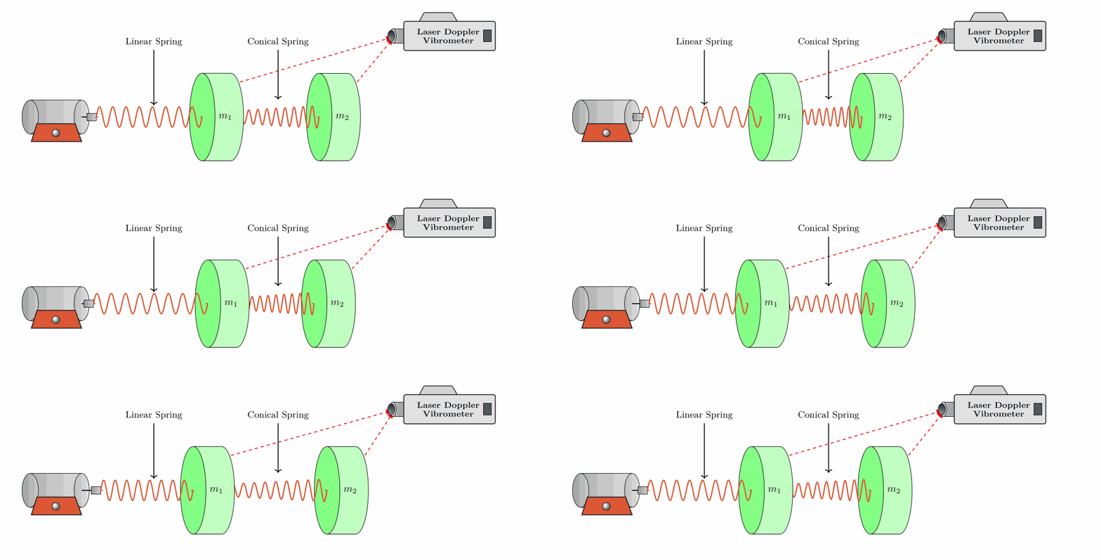
Theoretical Model

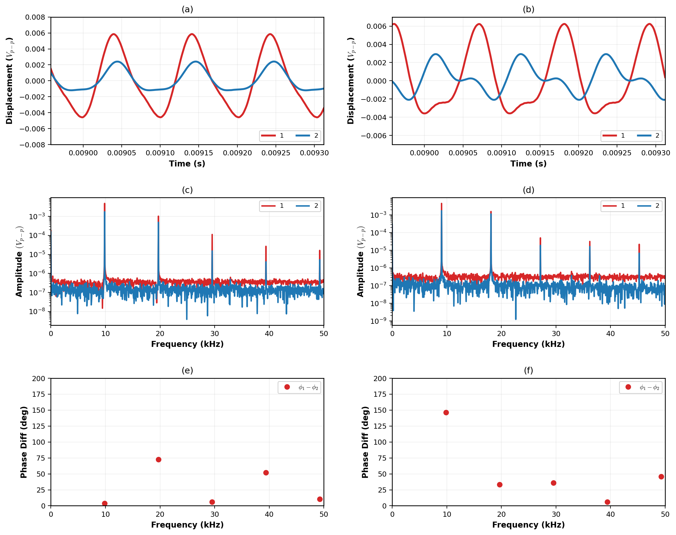
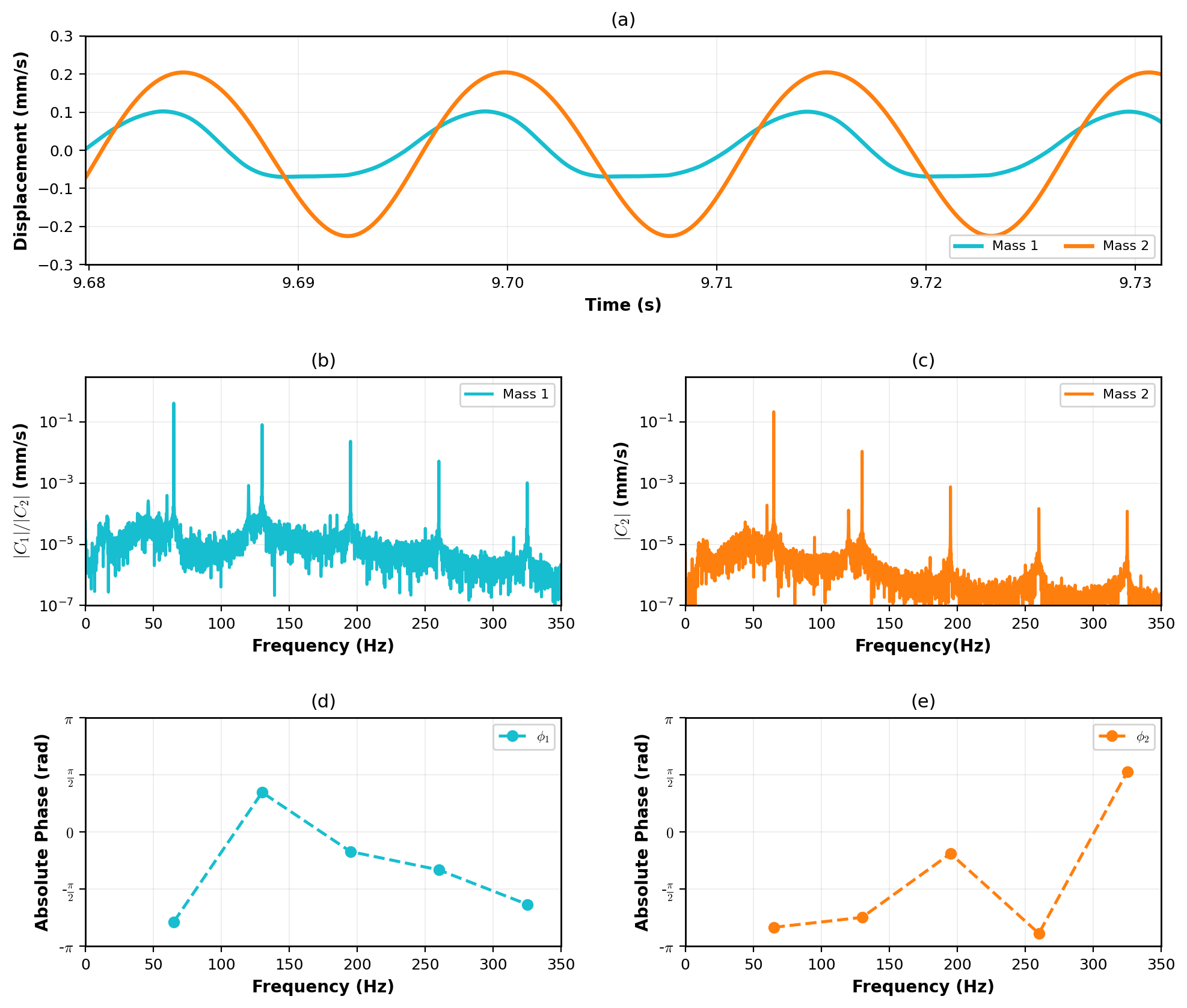
The experiment exhibits clear nonlinear behavior due to the conical spring, the analytical formulation used below retains the linear stiffness terms. Figs. 13 and 16 clearly show that the experimental mass-conical spring system exhibits nonlinear behavior. Because the conical springs behave differently in tension and compression, the motion over each vibration cycle can be separated into tension and compression segments. To model this, we use the following nonlinear formulation in which the restoring force includes higher-order displacement terms arising from the graded coil geometry. Thus, the governing equations of motion are written as

(52)\[\begin{equation} \begin{aligned} m_{1}^{\mathrm{eff}}\,\ddot{u}_1 &= k_1\!\left(F e^{i\omega_d t}-u_1\right) - k_2\left(u_1-u_2\right) - k_2^{\prime}\left(u_1 - u_2\right)_{+}^2 - k_2^{\prime\prime}\left(u_1 - u_2\right)_{+}^3 - \eta\,\dot{u}_1, \\ m_{2}^{\mathrm{eff}}\,\ddot{u}_2 &= - k_2\left(u_2-u_1\right) + k_2^{\prime}\left(u_1 - u_2\right)_{+}^2 + k_2^{\prime\prime}\left(u_1 - u_2\right)_{+}^3 - \eta\,\dot{u}_2. \end{aligned} \end{equation}\]

Here, \(m_{1}^{\mathrm{eff}}\) and \(m_{2}^{\mathrm{eff}}\) include the distributed mass of the springs based on \(m^{\mathrm{eff}} = m + m_k/3\) [Rao and Yap, 1995]. Because mass 1 connects to both springs, we write \(m_{1}^{\mathrm{eff}} = m + m_{k,1}/3 +m_{k,2}/3\), whereas for mass 2, \(m_{2}^{\mathrm{eff}} = m + m_{k,2}/3\). The variables \(u_1\) and \(u_2\) represent the displacements from equilibrium, \(F\) and \(\omega_d\) denote the drive amplitude and frequency, and \(\eta\) represents viscous damping. \(k_1\) is the stiffness of the linear spring connecting mass 1 to the shaker, and \(k_2\) is the nominal stiffness of the conical spring. The terms \(k_2^{\prime}\) and \(k_2^{\prime\prime}\) represent the quadratic and cubic nonlinear stiffness components. The Heaviside function \((\cdot)_{+}\) ensures that the nonlinear terms are activated only under compression.

Given the nonlinear nature of the mass–conical spring model, we employ a regular perturbation technique to obtain an approximate solution. Introducing a small, dimensionless parameter \(\epsilon\) (\(\epsilon \ll 1\)), Eq. (5) can be rewritten as

The nonlinear model can be rewritten by introducing a small dimensionless parameter \(\epsilon\) (\(\epsilon \ll 1\)) such that the nonlinear stiffness contributions enter at \(\mathcal{O}(\epsilon)\). Thus, the equations of motion take the form

(53)\[\begin{equation} \begin{aligned} m_1^{\mathrm{eff}}\,\ddot{u}_1 &= k_1\!\left( F e^{i\omega_d t} - u_1 \right) - k_2 \left( u_1 - u_2 \right) - \epsilon k_2^{\prime}\left( u_1 - u_2 \right)^2 - \epsilon k_2^{\prime\prime}\left( u_1 - u_2 \right)^3 - \eta\,\dot{u}_1, \\ m_2^{\mathrm{eff}}\,\ddot{u}_2 &= - k_2 \left( u_2 - u_1 \right) + \epsilon k_2^{\prime}\left( u_1 - u_2 \right)^2 + \epsilon k_2^{\prime\prime}\left( u_1 - u_2 \right)^3 - \eta\,\dot{u}_2. \end{aligned} \end{equation}\]

As the springs behave differently when it is tension or compression, we can divide the equation of motion into two different sections. In each vibrating period, there are compression and tension regions. Conical spring behaves nonlinearly when it is in compression. \(k_2^{'}\) and \(k_2^{''}\) are the quadratic and cubic nonlinear stiffness terms.

Relative Motion in Compression and Tension:

(54)\[\begin{equation} \Delta(t) = u_0(t) - v_0(t) = (A_0 - B_0)e^{i\omega_d t} \end{equation}\]

Here \(A_0\) and \(B_0\) are the amplitude response of the masses. This is the complex quantity with time varying real and imaginary parts, but the physical displacement is the real part:

(55)\[\begin{equation} \mathrm{Re}[\Delta(t)] = \mathrm{Re}[(A_0 - B_0)e^{i\omega_d t}] \end{equation}\]

Spring is in:

\[\begin{equation*} \text{Tension when }\mathrm{Re}[(A_0 - B_0)e^{i\omega_d t}] > 0 \end{equation*}\]

\[\begin{equation*} \text{Compression when }\mathrm{Re}[(A_0 - B_0)e^{i\omega_d t}] < 0 \end{equation*}\]

Let,

(56)\[\begin{equation} C = A_0 - B_0 = |C|e^{i\phi} \Rightarrow \mathrm{Re}[\Delta(t)] = |C|\cos(\omega_d t + \phi) \end{equation}\]

Since \(\cos\) is always symmetric and oscillatory, it always spans both positive and negative values, unless \(|C| = 0\), i.e., \(A_0 = B_0\). We want:

\[\begin{equation*} \mathrm{Re}[(A_0 - B_0)e^{i\omega_d t}] \ge 0 \text{ for all } t. \end{equation*}\]

That’s only possible if:

\[\begin{equation*} \mathrm{Im}[A_0 - B_0] = 0 \quad \text{and} \quad \mathrm{Re}[A_0 - B_0] > 0 \end{equation*}\]

And the exponential has no time-varying sign. So, the real part of the oscillation is constant and strictly positive. But this contradicts the nature of the harmonic forcing unless the two amplitudes are equal and real. So, in general: The spring is in compression during half the period and in tension during the other half, unless the phase and amplitude of \(A_0\) and \(B_0\) are tuned to suppress one side.

Let:

(57)\[\begin{equation} \Delta(t) = (A_0 - B_0)e^{i\omega_d t} \end{equation}\]

\[\begin{equation*} \Rightarrow \mathrm{Re}[\Delta(t)] = \mathrm{Re}[C]\cos(\omega_d t) - \mathrm{Im}[C]\sin(\omega_d t) \end{equation*}\]

So, define:

\[\begin{equation*} \mathrm{Re}[\Delta(t)] = R\cos(\omega_d t + \phi), \quad R = |C| \end{equation*}\]

Spring is in tension:

\[\begin{equation*} \cos(\omega_d t + \phi) > 0 \Rightarrow \omega_d t + \phi \in \left(-\frac{\pi}{2}, \frac{\pi}{2}\right) \end{equation*}\]

Spring is in compression:

\[\begin{equation*} \cos(\omega_d t + \phi) < 0 \Rightarrow \omega_d t + \phi \in \left(\frac{\pi}{2}, \frac{3\pi}{2}\right) \end{equation*}\]

Asymptotic Perturbation Solution of displacement:

(58)\[\begin{equation} u_1 = u_{1,0} + \epsilon u_{1,1} + \epsilon^2 u_{1,2}, \qquad u_2 = u_{2,0} + \epsilon u_{2,1} + \epsilon^2 u_{2,2} \end{equation}\]

Applying the solution to Eq. (51). We get,

(59)\[\begin{equation} \begin{aligned} m_1^{\mathrm{eff}}(\ddot{u}_{1,0} + \epsilon \ddot{u}_{1,1} + \epsilon^2 \ddot{u}_{1,2}) &= k_1(Fe^{i\omega_d t} - u_{1,0} - \epsilon u_{1,1} - \epsilon^2 u_{1,2}) \\ &\quad - k_2\!\left[(u_{1,0} - u_{2,0}) + \epsilon(u_{1,1} - u_{2,1}) + \epsilon^2(u_{1,2} - u_{2,2})\right] \\ &\quad - \epsilon k_2^{\prime}\!\left[(u_{1,0} - u_{2,0}) + \epsilon(u_{1,1} - u_{2,1}) + \epsilon^2(u_{1,2} - u_{2,2})\right]^2 \\ &\quad - \epsilon^2 k_2^{\prime\prime}\!\left[(u_{1,0} - u_{2,0}) + \epsilon(u_{1,1} - u_{2,1}) + \epsilon^2(u_{1,2} - u_{2,2})\right]^3 \\ &\quad - \eta(\dot{u}_{1,0} + \epsilon \dot{u}_{1,1} + \epsilon^2 \dot{u}_{1,2}) \\ m_2^{\mathrm{eff}}(\ddot{u}_{2,0} + \epsilon \ddot{u}_{2,1} + \epsilon^2 \ddot{u}_{2,2}) &= - k_2\!\left[(u_{2,0} - u_{1,0}) + \epsilon(u_{2,1} - u_{1,1}) + \epsilon^2(u_{2,2} - u_{1,2})\right] \\ &\quad - \epsilon k_2^{\prime}\!\left[(u_{2,0} - u_{1,0}) + \epsilon(u_{2,1} - u_{1,1}) + \epsilon^2(u_{2,2} - u_{1,2})\right]^2 \\ &\quad - \epsilon^2 k_2^{\prime\prime}\!\left[(u_{2,0} - u_{1,0}) + \epsilon(u_{2,1} - u_{1,1}) + \epsilon^2(u_{2,2} - u_{1,2})\right]^3 \\ &\quad - \eta(\dot{u}_{2,0} + \epsilon \dot{u}_{2,1} + \epsilon^2 \dot{u}_{2,2}) \end{aligned} \end{equation}\]

Let’s consider:

\[\begin{equation*} \Delta_0 = u_{1,0} - u_{2,0},\quad \Delta_1 = u_{1,1} - u_{2,1},\quad \Delta_2 = u_{1,2} - u_{2,2} \end{equation*}\]

Ignoring the higher power terms of \(\epsilon\), for mass 1, we get,

(60)\[\begin{equation} \begin{aligned} m_1^{\mathrm{eff}}(\ddot{u}_{1,0} + \epsilon \ddot{u}_{1,1} + \epsilon^2 \ddot{u}_{1,2}) &= k_1(Fe^{i\omega_d t} - u_{1,0} - \epsilon u_{1,1} - \epsilon^2 u_{1,2}) \\ &\quad - k_2(\Delta_0 + \epsilon\Delta_1 + \epsilon^2\Delta_2) \\ &\quad - \epsilon k_2^{\prime}(\Delta_0 + \epsilon\Delta_1)^2 - \epsilon^2 k_2^{\prime\prime}(\Delta_0)^3 \\ &\quad - \eta(\dot{u}_{1,0} + \epsilon \dot{u}_{1,1} + \epsilon^2 \dot{u}_{1,2}) \\ m_1^{\mathrm{eff}}(\ddot{u}_{1,0} + \epsilon \ddot{u}_{1,1} + \epsilon^2 \ddot{u}_{1,2}) &= [k_1(Fe^{i\omega_d t} - u_{1,0}) - k_2\Delta_0 - \eta \dot{u}_{1,0}] \\ &\quad + \epsilon[-k_1 u_{1,1} - k_2\Delta_1 - k_2^{\prime}\Delta_0^2 - \eta\dot{u}_{1,1}] \\ &\quad + \epsilon^2[-k_1 u_{1,2} - k_2\Delta_2 - 2k_2^{\prime}(\Delta_0 \Delta_1) - k_2^{\prime\prime}(\Delta_0^3) - \eta\dot{u}_{1,2}] \end{aligned} \end{equation}\]

Let’s consider:

\[\begin{equation*} \Delta_0 = u_{2,0} - u_{1,0},\quad \Delta_1 = u_{2,1} - u_{1,1},\quad \Delta_2 = u_{2,2} - u_{1,2} \end{equation*}\]

For Mass 2, we get,

(61)\[\begin{equation} \begin{aligned} m_2^{\mathrm{eff}}(\ddot{u}_{2,0} + \epsilon \ddot{u}_{2,1} + \epsilon^2 \ddot{u}_{2,2}) &= [-k_2(\Delta_0) - \eta\dot{u}_{2,0}] \\ &\quad + \epsilon[-k_2\Delta_1 - k_2^{\prime}\Delta_0^2 - \eta\dot{u}_{2,1}] \\ &\quad + \epsilon^2[-k_2\Delta_2 - 2k_2^{\prime}(\Delta_0 \Delta_2) - k_2^{\prime\prime}\Delta_0^3 - \eta\dot{u}_{2,2}] \end{aligned} \end{equation}\]

The Equation of Motion for each order of displacement is,

\[\begin{flalign*} \epsilon^0:\quad m_1^{\mathrm{eff}} \ddot{u}_{1,0} &= k_1\left(Fe^{i\omega_d t} - u_{1,0}\right) - k_2\left(u_{1,0} - u_{2,0}\right) - \eta \dot{u}_{1,0} && \\ m_2^{\mathrm{eff}} \ddot{u}_{2,0} &= -k_2\left(u_{2,0} - u_{1,0}\right) - \eta \dot{u}_{2,0} && \end{flalign*}\]

\[\begin{flalign*} \epsilon^1:\quad m_1^{\mathrm{eff}} \ddot{u}_{1,1} &= -k_1 u_{1,1} - k_2\left(u_{2,1} - u_{1,1}\right) - k_2^{\prime}\left(u_{1,0} - u_{2,0}\right)^2 - \eta \dot{u}_{1,1} && \\ m_2^{\mathrm{eff}} \ddot{u}_{2,1} &= -k_2\left(u_{2,1} - u_{1,1}\right) - k_2^{\prime}\left(u_{2,0} - u_{1,0}\right)^2 - \eta \dot{u}_{2,1} && \end{flalign*}\]

Let’s consider the solution of the displacement term as,

\[\begin{equation*} \dot{u}_{1,n-1} = i\omega_d C_{1,n-1} e^{i\omega_d t},\qquad \dot{u}_{2,n-1} = i\omega_d C_{2,n-1} e^{i\omega_d t} \end{equation*}\]

\[\begin{equation*} \ddot{u}_{1,n-1} = -\omega_d^2 C_{1,n-1} e^{i\omega_d t},\qquad \ddot{u}_{2,n-1} = -\omega_d^2 C_{2,n-1} e^{i\omega_d t} \end{equation*}\]

We apply this in the equation, then we get,

\[\begin{equation*} -m_1^{\mathrm{eff}} \omega_d^2 C_{1,0} e^{i\omega_d t} = k_1\left(Fe^{i\omega_d t} - C_{1,0} e^{i\omega_d t}\right) - k_2\left(C_{1,0} e^{i\omega_d t} - C_{2,0} e^{i\omega_d t}\right) - i\eta\omega_d C_{1,0} e^{i\omega_d t} \end{equation*}\]

\[\begin{equation*} \Rightarrow -m_1^{\mathrm{eff}} \omega_d^2 C_{1,0} = k_1(F - C_{1,0}) - k_2(C_{1,0} - C_{2,0}) - i\eta\omega_d C_{1,0} \end{equation*}\]

\[\begin{equation*} \Rightarrow (-m_1^{\mathrm{eff}} \omega_d^2 + k_1 + k_2 + i\eta\omega_d) C_{1,0} - k_2 C_{2,0} = k_1 F \end{equation*}\]

\[\begin{equation*} -m_2^{\mathrm{eff}} \omega_d^2 C_{2,0} e^{i\omega_d t} = k_2\left(C_{1,0} e^{i\omega_d t} - C_{2,0} e^{i\omega_d t}\right) - i\eta\omega_d C_{2,0} e^{i\omega_d t} \end{equation*}\]

\[\begin{equation*} \Rightarrow -m_2^{\mathrm{eff}} \omega_d^2 C_{2,0} = k_2(C_{1,0} - C_{2,0}) - i\eta\omega_d C_{2,0} \end{equation*}\]

\[\begin{equation*} \Rightarrow -k_2 C_{1,0} + (-m_2^{\mathrm{eff}} \omega_d^2 + k_2 + i\eta\omega_d) C_{2,0} = 0 \end{equation*}\]

The amplitude of zeroth order displacement is,

\[\begin{equation*} C_{1,0} = \frac{k_1 F(-m_2^{\mathrm{eff}} \omega_d^2 + k_2 + i\eta\omega_d)} {(-m_1^{\mathrm{eff}} \omega_d^2 + k_1 + k_2 + i\eta\omega_d)(-m_2^{\mathrm{eff}} \omega_d^2 + k_2 + i\eta\omega_d) - k_2^2} \end{equation*}\]

\[\begin{equation*} C_{2,0} = \frac{k_1 k_2 F} {(-m_1^{\mathrm{eff}} \omega_d^2 + k_1 + k_2 + i\eta\omega_d)(-m_2^{\mathrm{eff}} \omega_d^2 + k_2 + i\eta\omega_d) - k_2^2} \end{equation*}\]

For the case of first order amplitude, we get,

\[\begin{equation*} m_1^{\mathrm{eff}} \ddot{u}_{1,1} = -k_1 u_{1,1} - k_2(u_{2,1} - u_{1,1}) - k_2^{\prime}(u_{1,0} - u_{2,0})^2 - \eta \dot{u}_{1,1} \end{equation*}\]

\[\begin{equation*} m_2^{\mathrm{eff}} \ddot{u}_{2,1} = -k_2(u_{2,1} - u_{1,1}) - k_2^{\prime}(u_{2,0} - u_{1,0})^2 - \eta \dot{u}_{2,1} \end{equation*}\]

Using substitution method and applying solution of \(u_1\) and \(u_2\), we get,

\[\begin{equation*} -8m_1^{\mathrm{eff}} \omega_d^2 C_{1,1} e^{2i\omega_d t} = -k_1 (2C_{1,1} e^{2i\omega_d t}) -k_2 (2C_{1,1} e^{2i\omega_d t}-2C_{2,1} e^{2i\omega_d t}) -k_2^{\prime} (C_{1,0} e^{i\omega_d t}-C_{2,0} e^{i\omega_d t})^2 -4i\eta\omega_d C_{1,1} e^{2i\omega_d t} \end{equation*}\]

\[\begin{equation*} \Rightarrow -8m_1^{\mathrm{eff}} \omega_d^2 C_{1,1} e^{2i\omega_d t} = -k_1 (2C_{1,1}) e^{2i\omega_d t} -2k_2 (C_{1,1}-C_{2,1}) e^{2i\omega_d t} -k_2^{\prime} (C_{1,0}-C_{2,0})^2 e^{2i\omega_d t} -4i\eta\omega_d C_{1,1} e^{2i\omega_d t} \end{equation*}\]

\[\begin{equation*} \Rightarrow -8m_1^{\mathrm{eff}} \omega_d^2 C_{1,1} = -2k_1 C_{1,1} -2k_2(C_{1,1}-C_{2,1}) -k_2^{\prime}(C_{1,0}-C_{2,0})^2 -4i\eta\omega_d C_{1,1} \end{equation*}\]

\[\begin{equation*} \Rightarrow (-8m_1^{\mathrm{eff}} \omega_d^2+2k_1+2k_2+4i\eta\omega_d)\,C_{1,1} -2k_2 C_{2,1} = k_2^{\prime}(C_{1,0}-C_{2,0})^2 \end{equation*}\]

And

\[\begin{equation*} -8m_2^{\mathrm{eff}} \omega_d^2 C_{2,1} e^{2i\omega_d t} = -k_2(2C_{2,1} e^{2i\omega_d t}-2C_{1,1} e^{2i\omega_d t}) -k_2^{\prime}(C_{2,0} e^{i\omega_d t}-C_{1,0} e^{i\omega_d t})^2 -4i\eta\omega_d C_{2,1} e^{2i\omega_d t} \end{equation*}\]

\[\begin{equation*} \Rightarrow -8m_2^{\mathrm{eff}} \omega_d^2 C_{2,1} e^{2i\omega_d t} = -k_2(2C_{2,1}-2C_{1,1}) e^{2i\omega_d t} -k_2^{\prime}(C_{2,0}-C_{1,0})^2 e^{2i\omega_d t} -4i\eta\omega_d C_{2,1} e^{2i\omega_d t} \end{equation*}\]

\[\begin{equation*} \Rightarrow -8m_2^{\mathrm{eff}} \omega_d^2 C_{2,1} = 2k_2(C_{1,1}-C_{2,1}) -k_2^{\prime}(C_{2,0}-C_{1,0})^2 -4i\eta\omega_d C_{2,1} \end{equation*}\]

\[\begin{equation*} \Rightarrow -2k_2 C_{1,1} +(-8m_2^{\mathrm{eff}} \omega_d^2+2k_2+4i\eta\omega_d)\,C_{2,1} = k_2^{\prime}(C_{1,0}-C_{2,0})^2 \end{equation*}\]

Using elimination method, we get,

\[\begin{equation*} C_{1,1} = \frac{ k_2^{\prime}(C_{1,0}-C_{2,0})^2\left((-8m_2^{\mathrm{eff}} \omega_d^2+2k_2+4i\eta\omega_d)+2k_2\right) }{ (-8m_1^{\mathrm{eff}} \omega_d^2+2k_1+2k_2+4i\eta\omega_d)(-8m_2^{\mathrm{eff}} \omega_d^2+2k_2+4i\eta\omega_d)-4k_2^2 } \end{equation*}\]

\[\begin{equation*} C_{2,1} = \frac{ k_2^{\prime}(C_{1,0}-C_{2,0})^2\left((-8m_1^{\mathrm{eff}} \omega_d^2+2k_1+2k_2+4i\eta\omega_d)+2k_2\right) }{ (-8m_1^{\mathrm{eff}} \omega_d^2+2k_1+2k_2+4i\eta\omega_d)(-8m_2^{\mathrm{eff}} \omega_d^2+2k_2+4i\eta\omega_d)-4k_2^2 } \end{equation*}\]

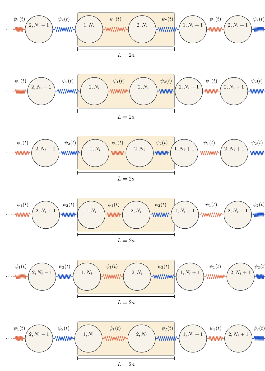
To elucidate the measured trends for Bit 1, we linearize the two-mass, two-spring dimer:

(62)\[\begin{equation} \begin{aligned} m_1^{\mathrm{eff}} \ddot{u}_1 &= k_1 (F e^{i\omega_d t} - u_1) - k_2 (u_1 - u_2) - \eta \dot{u}_1, \\ m_2^{\mathrm{eff}} \ddot{u}_2 &= k_2 (u_1 - u_2) - \eta \dot{u}_2. \end{aligned} \end{equation}\]

Here, \(m_1^{\mathrm{eff}}\) and \(m_2^{\mathrm{eff}}\) include the spring mass via \(m^{\mathrm{eff}} = m + m_k/3\) [Rao and Yap, 1995]. Because Mass 1 is connected to both springs, \(m_1^{\mathrm{eff}} = m + m_{k,1}/3 + m_{k,2}/3\), whereas for Mass 2, \(m_2^{\mathrm{eff}} = m + m_{k,2}/3\). \(u_1\) and \(u_2\) represent the displacements of the masses from equilibrium. \(F\) and \(\omega_d\) denote the driver amplitude and frequency, respectively, \(\eta\) represents viscous damping, \(k_1\) is the stiffness of the linear spring connecting the first mass to the driver, and \(k_2\) is the stiffness of the inter-mass conical spring.

Assuming harmonic motion \(u_1 = C_1 e^{i\omega_d t}\) and \(u_2 = C_2 e^{i\omega_d t}\) with complex amplitudes \(C_1\) and \(C_2\), substituting into Eq. (60) yields the algebraic system,

The linearized model for the mass-spring system is considered in Eq. (60), and the assumed harmonic ansatz for the displacement fields is

\[\begin{equation*} u_1 = C_1 e^{i\omega_d t}, \qquad u_2 = C_2 e^{i\omega_d t}. \end{equation*}\]

The first and second derivatives with respect to time are

\[\begin{equation*} \dot{u}_1 = i\omega_d C_1 e^{i\omega_d t}, \quad \dot{u}_2 = i\omega_d C_2 e^{i\omega_d t}, \qquad \ddot{u}_1 = -\omega_d^2 C_1 e^{i\omega_d t}, \quad \ddot{u}_2 = -\omega_d^2 C_2 e^{i\omega_d t}. \end{equation*}\]

Substituting these expressions into Eq. (60) gives

(63)\[\begin{equation} \begin{aligned} &-m_1^{\mathrm{eff}}\omega_d^2 C_1 e^{i\omega_d t} = k_1\!\left(F e^{i\omega_d t} - C_1 e^{i\omega_d t}\right) - k_2\!\left(C_1 e^{i\omega_d t} - C_2 e^{i\omega_d t}\right) - i\eta\omega_d C_1 e^{i\omega_d t}, \\[4pt] \Rightarrow & \; -m_1^{\mathrm{eff}}\omega_d^2 C_1 e^{i\omega_d t} = \big[k_1(F - C_1) - k_2(C_1 - C_2) - i\eta\omega_d C_1\big] e^{i\omega_d t}, \\[4pt] \Rightarrow \; &-m_1^{\mathrm{eff}}\omega_d^2 C_1 = k_1(F - C_1) - k_2(C_1 - C_2) - i\eta\omega_d C_1, \\[4pt] \Rightarrow & \; (-m_1^{\mathrm{eff}}\omega_d^2 + k_1 + k_2 + i\eta\omega_d)C_1 - k_2 C_2 = k_1 F.\\ &-m_2^{\mathrm{eff}}\omega_d^2 C_2 e^{i\omega_d t} = k_2\!\left(C_1 e^{i\omega_d t} - C_2 e^{i\omega_d t}\right) - i\eta\omega_d C_2 e^{i\omega_d t}, \\[4pt] \Rightarrow & \; -m_2^{\mathrm{eff}}\omega_d^2 C_2 e^{i\omega_d t} = \big[k_2(C_1 - C_2) - i\eta\omega_d C_2\big] e^{i\omega_d t}, \\[4pt] \Rightarrow & \; -m_2^{\mathrm{eff}}\omega_d^2 C_2 = k_2(C_1 - C_2) - i\eta\omega_d C_2, \\[4pt] \Rightarrow & \; -k_2 C_1 + (-m_2^{\mathrm{eff}}\omega_d^2 + k_2 + i\eta\omega_d)C_2 = 0. \end{aligned} \end{equation}\]

Solving the above equations yields the amplitude responses of the two masses and the eigenmode frequencies.

(64)\[\begin{equation} \begin{aligned} C_1 &= \frac{k_1 F \left(-m_2^{\mathrm{eff}} \omega_d^2 + k_2 + i\eta\omega_d\right)} {\left(-m_1^{\mathrm{eff}} \omega_d^2 + k_1 + k_2 + i\eta\omega_d\right) \left(-m_2^{\mathrm{eff}} \omega_d^2 + k_2 + i\eta\omega_d\right) - k_2^2}, \\[4pt] C_2 &= \frac{k_1 k_2 F} {\left(-m_1^{\mathrm{eff}} \omega_d^2 + k_1 + k_2 + i\eta\omega_d\right) \left(-m_2^{\mathrm{eff}} \omega_d^2 + k_2 + i\eta\omega_d\right) - k_2^2}. \end{aligned} \end{equation}\]

The algebraic solution of the masses are written as the stiffness matrix as,

\[\begin{equation*} \begin{bmatrix} -m_1^{\mathrm{eff}}\omega_d^2 + k_1 + k_2 & -k_2 \\[3pt] -k_2 & -m_2^{\mathrm{eff}}\omega_d^2 + k_2 \end{bmatrix} \end{equation*}\]

The eigenmode frequency is taken as the determinant of the stiffness matrix as \(\det(K)=0\). This can be implemented by taking the real part of the stiffness matrix as (the eigenmode of the system does not come from the damping provided in the system),

(65)\[\begin{equation} \begin{aligned} &\det \begin{bmatrix} -m_1^{\mathrm{eff}}\omega_d^2 + k_1 + k_2 & -k_2 \\[3pt] -k_2 & -m_2^{\mathrm{eff}}\omega_d^2 + k_2 \end{bmatrix} = 0, \\[6pt] &(-m_1^{\mathrm{eff}}\omega_d^2 + k_1 + k_2) (-m_2^{\mathrm{eff}}\omega_d^2 + k_2) - k_2^2 = 0, \\[6pt] &m_1^{\mathrm{eff}}m_2^{\mathrm{eff}}\omega_d^4 - m_1^{\mathrm{eff}}k_2\omega_d^2 - m_2^{\mathrm{eff}}(k_1 + k_2)\omega_d^2 - k_2^2 = 0, \\[6pt] &m_1^{\mathrm{eff}}m_2^{\mathrm{eff}}\omega_d^4 - \omega_d^2\!\left(m_1^{\mathrm{eff}}k_2 + m_2^{\mathrm{eff}}k_1 + m_2^{\mathrm{eff}}k_2\right) + k_2(k_1 + k_2) - k_2^2 = 0, \\[6pt] \quad &m_1^{\mathrm{eff}}m_2^{\mathrm{eff}}\omega_d^4 - \omega_d^2\!\left(m_1^{\mathrm{eff}}k_2 + m_2^{\mathrm{eff}}k_1 + m_2^{\mathrm{eff}}k_2\right) + k_1k_2 = 0. \end{aligned} \end{equation}\]

Using the quadratic formula \(x = \frac{B \pm \sqrt{B^2 - 4AC}}{2A}\), the two roots of Eq. (63) yield the eigenmode frequencies,

(66)\[\begin{equation} \omega_{01,02}^2 = \frac{ m_1^{\mathrm{eff}} k_2 + m_2^{\mathrm{eff}}(k_1 + k_2) \pm \sqrt{ \left[m_1^{\mathrm{eff}} k_2 + m_2^{\mathrm{eff}}(k_1 + k_2)\right]^2 - 4 m_1^{\mathrm{eff}} m_2^{\mathrm{eff}} k_1 k_2 } }{2 m_1^{\mathrm{eff}} m_2^{\mathrm{eff}}}. \end{equation}\]

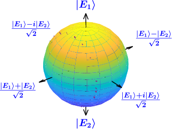
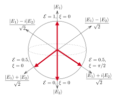
Substituting these into the stiffness matrix provides the corresponding eigenvectors, or eigenstates, of the dimer:

\[\begin{equation*} \ket{E_1} = \frac{1}{\sqrt{2}}\begin{pmatrix}1\\1\end{pmatrix}, \qquad \ket{E_2} = \frac{1}{\sqrt{2}}\begin{pmatrix}1\\-1\end{pmatrix}. \end{equation*}\]

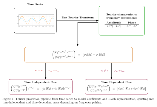
Applying the amplitude responses \(C_1\) and \(C_2\) to this orthonormal basis, the vibrational state vector of the system is written as

(67)\[\begin{equation} \mathbf{U}= \begin{bmatrix} C_1 \\ C_2 \end{bmatrix} \equiv \psi_0 \ket{E_1} + \psi_1 \ket{E_2} = \frac{1}{\sqrt{2}}\,\psi_0 \begin{bmatrix} 1 \\ 1 \end{bmatrix} + \frac{1}{\sqrt{2}}\,\psi_1 \begin{bmatrix} 1 \\ -1 \end{bmatrix}= \frac{1}{\sqrt{2}} \begin{bmatrix} \psi_0 + \psi_1 \\ \psi_0 - \psi_1 \end{bmatrix}. \end{equation}\]

We can calculate the coefficients of the superposition of states from the orthonormal basis of the eigenstates (\(\psi_{(0,d)}\) and \(\psi_{(1,d)}\)) for the linearized model at the fundamental characteristics of the masses. This can be written as

(68)\[\begin{equation} \begin{aligned} \psi_0 = \frac{C_1 + C_2}{\sqrt{2}} &= \frac{1}{\sqrt{2}} \bigg[ \frac{k_1 F(-m_2^{\mathrm{eff}}\omega_d^2 + k_2 + i\eta\omega_d)} {(-m_1^{\mathrm{eff}}\omega_d^2 + k_1 + k_2 + i\eta\omega_d) (-m_2^{\mathrm{eff}}\omega_d^2 + k_2 + i\eta\omega_d) - k_2^2} \\[4pt] &\qquad + \frac{k_1 k_2 F} {(-m_1^{\mathrm{eff}}\omega_d^2 + k_1 + k_2 + i\eta\omega_d) (-m_2^{\mathrm{eff}}\omega_d^2 + k_2 + i\eta\omega_d) - k_2^2} \bigg] \\[6pt] &= \frac{1}{\sqrt{2}} \bigg[ \frac{k_1 F(-m_2^{\mathrm{eff}}\omega_d^2 + k_2 + i\eta\omega_d) + k_1 k_2 F} {(-m_1^{\mathrm{eff}}\omega_d^2 + k_1 + k_2 + i\eta\omega_d) (-m_2^{\mathrm{eff}}\omega_d^2 + k_2 + i\eta\omega_d) - k_2^2} \bigg] \\[6pt] &= \frac{1}{\sqrt{2}} \bigg[ \frac{k_1 F(-m_2^{\mathrm{eff}}\omega_d^2 + 2k_2 + i\eta\omega_d)} {(-m_1^{\mathrm{eff}}\omega_d^2 + k_1 + k_2 + i\eta\omega_d) (-m_2^{\mathrm{eff}}\omega_d^2 + k_2 + i\eta\omega_d) - k_2^2} \bigg], \\[12pt] \psi_1 = \frac{C_1 - C_2}{\sqrt{2}} &= \frac{1}{\sqrt{2}} \bigg[ \frac{k_1 F(-m_2^{\mathrm{eff}}\omega_d^2 + k_2 + i\eta\omega_d)} {(-m_1^{\mathrm{eff}}\omega_d^2 + k_1 + k_2 + i\eta\omega_d) (-m_2^{\mathrm{eff}}\omega_d^2 + k_2 + i\eta\omega_d) - k_2^2} \\[4pt] &\qquad - \frac{k_1 k_2 F} {(-m_1^{\mathrm{eff}}\omega_d^2 + k_1 + k_2 + i\eta\omega_d) (-m_2^{\mathrm{eff}}\omega_d^2 + k_2 + i\eta\omega_d) - k_2^2} \bigg] \\[6pt] &= \frac{1}{\sqrt{2}} \bigg[ \frac{k_1 F(-m_2^{\mathrm{eff}}\omega_d^2 + k_2 + i\eta\omega_d) - k_1 k_2 F} {(-m_1^{\mathrm{eff}}\omega_d^2 + k_1 + k_2 + i\eta\omega_d) (-m_2^{\mathrm{eff}}\omega_d^2 + k_2 + i\eta\omega_d) - k_2^2} \bigg] \\[6pt] &= \frac{1}{\sqrt{2}} \bigg[ \frac{k_1 F(-m_2^{\mathrm{eff}}\omega_d^2 + i\eta\omega_d)} {(-m_1^{\mathrm{eff}}\omega_d^2 + k_1 + k_2 + i\eta\omega_d) (-m_2^{\mathrm{eff}}\omega_d^2 + k_2 + i\eta\omega_d) - k_2^2} \bigg]. \end{aligned} \end{equation}\]

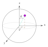
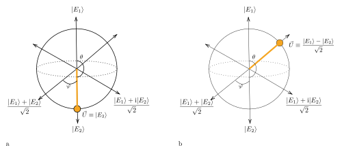
\(\psi_0\) and \(\psi_1\) represent the coefficients of the superposition of states at the driving frequency \((\omega_d)\). The Bloch states angle can also be derived from the coefficients such that, \(\theta = 2\cos^{-1}(|\psi_0|).\) From Eq. (66), let \(D = (-m_1^{\mathrm{eff}} \omega_d^2 + k_1 + k_2 + i \eta \omega_d)(-m_2^{\mathrm{eff}} \omega_d^2 + k_2 + i \eta \omega_d) - k_2^2.\) So, the simplified equation becomes,

(69)\[\begin{equation} \theta = 2 \cos^{-1}\!\left( \left|\frac{1}{\sqrt{2}} \frac{k_1 F}{D} (-m_2^{\mathrm{eff}} \omega_d^2 + 2k_2 + i \eta \omega_d)\right| \right) = 2 \cos^{-1}\!\left( \left|\frac{k_1 F}{\sqrt{2} D}\right| \sqrt{(-m_2^{\mathrm{eff}} \omega_d^2 + 2k_2)^2 + \eta^2 \omega_d^2} \right). \end{equation}\]

Similarly, the azimuthal angle of the Bloch states, \(\varphi = \arg(\psi_0) - \arg(\psi_1).\) The simplified equation becomes,

(70)\[\begin{equation} \arg(\psi_0) = \arg\!\left( \frac{1}{\sqrt{2}} \frac{k_1 F(-m_2^{\mathrm{eff}} \omega_d^2 + 2k_2 + i \eta \omega_d)} {(-m_1^{\mathrm{eff}} \omega_d^2 + k_1 + k_2 + i \eta \omega_d) (-m_2^{\mathrm{eff}} \omega_d^2 + k_2 + i \eta \omega_d) - k_2^2} \right). \end{equation}\]

Let the numerator \(N = k_1 F(-m_2^{\mathrm{eff}} \omega_d^2 + 2k_2 + i \eta \omega_d),\) This is the product of the real constants and a complex number. Fundamental property of the argument of a complex number suggests that, for any two complex numbers, the argument of their product is the sum of their arguments. In that case,

\[\begin{equation*} \arg(k_1 F(-m_2^{\mathrm{eff}} \omega_d^2 + 2k_2 + i \eta \omega_d)) = \arg(k_1 F) + \arg(-m_2^{\mathrm{eff}} \omega_d^2 + 2k_2 + i \eta \omega_d) = \arg(k_1 F) + \tan^{-1}\!\left(\frac{\eta \omega_d}{-m_2^{\mathrm{eff}} \omega_d^2 + 2k_2}\right). \end{equation*}\]

And let the denominator \(D = (-m_1^{\mathrm{eff}} \omega_d^2 + k_1 + k_2 + i \eta \omega_d)(-m_2^{\mathrm{eff}} \omega_d^2 + k_2 + i \eta \omega_d) - k_2^2\). So, the argument of the coefficient \(\psi_0\) is,

\[\begin{equation*} \arg(\psi_0) = \arg(k_1 F) + \tan^{-1}\!\left(\frac{\eta \omega_d}{-m_2^{\mathrm{eff}} \omega_d^2 + 2k_2}\right) - \arg(D). \end{equation*}\]

Similarly, for the case of \(\psi_1\), we get the phase of that term as,

\[\begin{equation*} \arg(\psi_1) = \arg(k_1 F) + \tan^{-1}\left(\frac{\eta \omega_d}{-m_2^{\mathrm{eff}} \omega_d^2}\right) - \arg(D). \end{equation*}\]

The azimuthal angle \(\varphi\) for the linearized model can be written as,

(71)\[\begin{equation} \begin{aligned} \varphi &= \arg(\psi_0) - \arg(\psi_1) \\ &= \arg(k_1 F) + \tan^{-1}\!\left(\frac{\eta \omega_d}{-m_2^{\mathrm{eff}} \omega_d^2 + 2k_2}\right) - \arg(D) - \arg(k_1 F) - \tan^{-1}\!\left(\frac{\eta \omega_d}{-m_2^{\mathrm{eff}} \omega_d^2}\right) + \arg(D) \\ &= \tan^{-1}\!\left(\frac{\eta \omega_d}{-m_2^{\mathrm{eff}} \omega_d^2 + 2k_2}\right) - \tan^{-1}\!\left(\frac{\eta \omega_d}{-m_2^{\mathrm{eff}} \omega_d^2}\right) \\ &= \tan^{-1}\!\left( \frac{ \frac{\eta \omega_d}{-m_2^{\mathrm{eff}} \omega_d^2 + 2k_2} - \frac{\eta \omega_d}{-m_2^{\mathrm{eff}} \omega_d^2} }{ \frac{\eta \omega_d}{-m_2^{\mathrm{eff}} \omega_d^2 + 2k_2} \frac{\eta \omega_d}{-m_2^{\mathrm{eff}} \omega_d^2} } \right) \\ &= \tan^{-1}\!\left( \frac{ (-m \eta \omega_d^3 + m \eta \omega_d^3 - 2k_2 \eta \omega_d) }{ (-m_2^{\mathrm{eff}} \omega_d^2 + 2k_2)(-m_2^{\mathrm{eff}} \omega_d^2) } \bigg/ \frac{ (-m_2^{\mathrm{eff}} \omega_d^2 + 2k_2)(-m_2^{\mathrm{eff}} \omega_d^2) + \eta^2 \omega_d^2 }{ (-m_2^{\mathrm{eff}} \omega_d^2 + 2k_2)(-m_2^{\mathrm{eff}} \omega_d^2) } \right) \\ &= \tan^{-1}\!\left( \frac{-2 k_2 \eta \omega_d}{ (-m_2^{\mathrm{eff}} \omega_d^2 + 2k_2)(-m_2^{\mathrm{eff}} \omega_d^2) + \eta^2 \omega_d^2} \right). \end{aligned} \end{equation}\]

so the polar and azimuthal angle at bit 1 is:

(72)\[\begin{equation} \begin{aligned} \theta(\omega_d) &= 2\cos^{-1}\left( \left|\psi_{(0,d)}\right| \right) = 2\cos^{-1}\Bigg[ \frac{ |k_1 F| }{ \sqrt{2}\,|D| } \sqrt{ \left(-m_2^{\mathrm{eff}}\omega_d^2 + 2k_2\right)^2 + (\eta\omega_d)^2 } \Bigg] \\ \varphi(\omega_d) &= \arg(\psi_{(0,d)}) - \arg(\psi_{(1,d)}) = \tan^{-1}\left( \frac{ -2k_2\,\eta\omega_d }{ (-m_2^{\mathrm{eff}}\omega_d^2 + 2k_2)(-m_2^{\mathrm{eff}}\omega_d^2) + \eta^2\omega_d^2 } \right) \end{aligned} \end{equation}\]

The dynamic behavior of Bit 2 is governed by the evolution of the polar angle \(\theta\) and azimuthal angle \(\phi\), which are directly influenced by the vibration mode of the connecting spring. Notably, the spring exhibits a piecewise stiffness behavior: it responds linearly when in tension and nonlinearly when in compression. This intrinsic asymmetric introduces a mechanism by which nonlinear modal behavior can be selectively excited or suppressed depending on the amplitude and phase difference between mass displacements.

(73)\[\begin{equation} \begin{aligned} \psi_{(0,2\omega_d)} = \frac{1}{\sqrt{2}}\, \frac{ k_2^{\prime} (C_{1,0}-C_{2,0})^2 \left[-8(m_1^{\mathrm{eff}}+m_2^{\mathrm{eff}})\omega_d^2 + 2k_1 + 8k_2 + 8i\eta\omega_d\right] }{ (-8m_1^{\mathrm{eff}}\omega_d^2 + 2k_1 + 2k_2 + 4i\eta\omega_d) (-8m_2^{\mathrm{eff}}\omega_d^2 + 2k_2 + 4i\eta\omega_d) - 4k_2^2 } \\ \psi_{(1,2\omega_d)} = \frac{1}{\sqrt{2}}\, \frac{ k_2^{\prime}(C_{1,0}-C_{2,0})^2 \left[-8(m_2^{\mathrm{eff}}-m_1^{\mathrm{eff}})\omega_d^2 - 2k_1\right] }{ (-8m_1^{\mathrm{eff}}\omega_d^2 + 2k_1 + 2k_2 + 4i\eta\omega_d) (-8m_2^{\mathrm{eff}}\omega_d^2 + 2k_2 + 4i\eta\omega_d) - 4k_2^2 } \end{aligned} \end{equation}\]

and the polar and azimuthal angle

(74)\[\begin{equation} \begin{aligned} \theta(2\omega_d) &= 2\cos^{-1}\Bigg[ \frac{ |k_2^{\prime}|\,|C_1^{\prime} - C_2^{\prime}|^2 }{ \sqrt{2}\,V } \sqrt{ \left(-8(m_1^{\mathrm{eff}} + m_2^{\mathrm{eff}})\omega_d^2 + 2k_1 + 8k_2\right)^2 + (8i\eta\omega_d)^2 } \Bigg] \\ \varphi(2\omega_d) &= \tan^{-1}\left[ \frac{ 8\eta\omega_d }{ -8(m_1^{\mathrm{eff}} + m_2^{\mathrm{eff}})\omega_d^2 + 2k_1 + 8k_2 } \right] - \arg\left[ 8(m_1^{\mathrm{eff}} - m_2^{\mathrm{eff}})\omega_d^2 - 2k_1 \right] \end{aligned} \end{equation}\]

Figure. Theoretical Analogy of the Frequency Dependent Evolution of the Bloch States of Elastic Bit 1 and 2. (a) Analytical prediction of Bit 1 obtained from the zeroth order (\(\epsilon^0\)) model [Eq. (70)], reproducing both the \(\theta\) sweep and the \(\varphi\) jump with an adjustable damping parameter. (b) Analytical prediction of Bit 2 obtained from the first order (\(\epsilon^1\)) model [Eq. (72)].

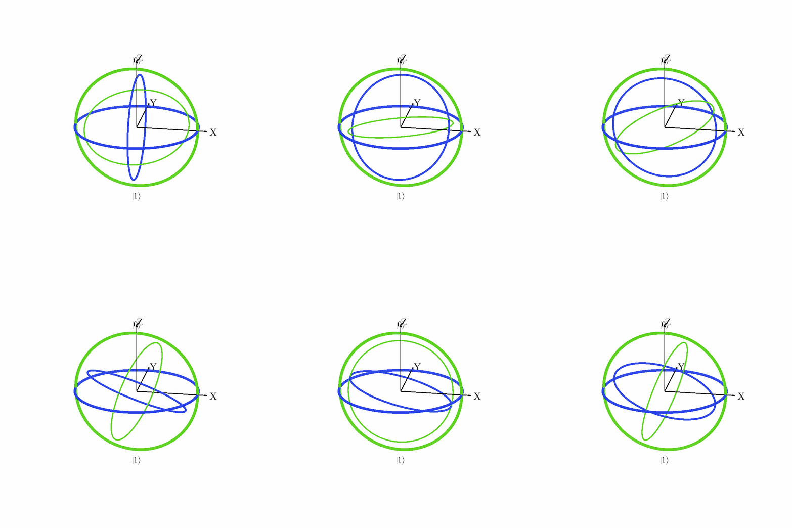
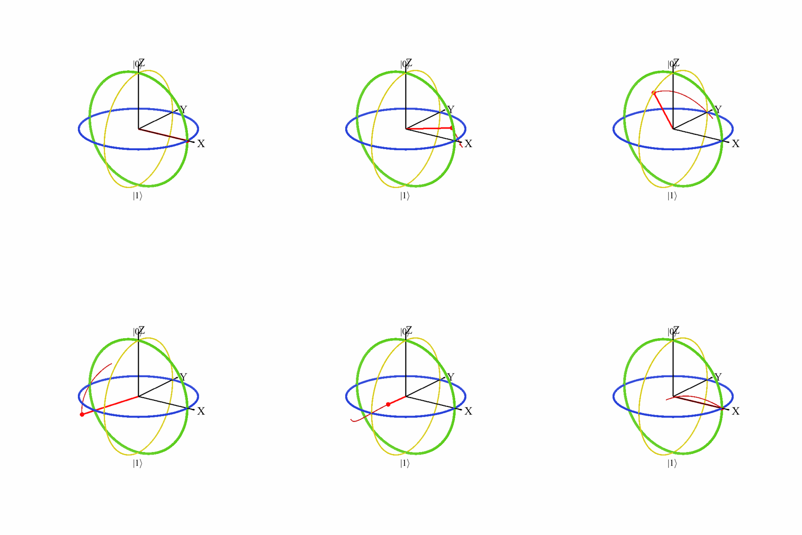
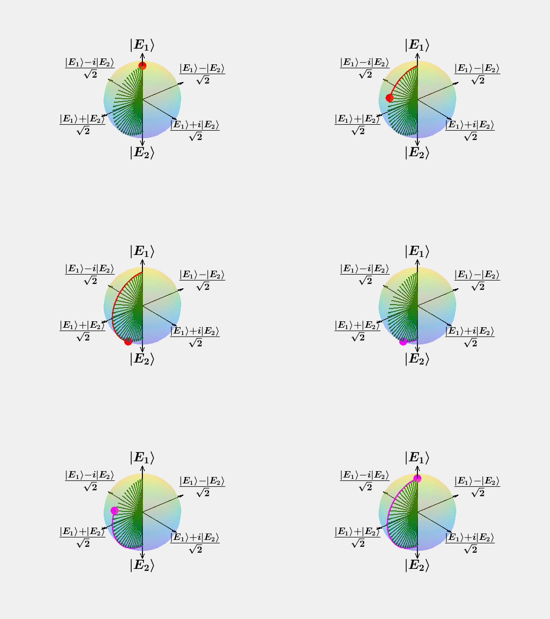
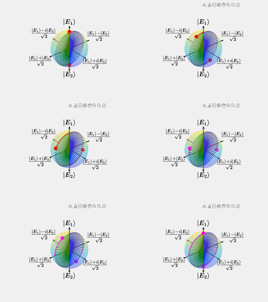
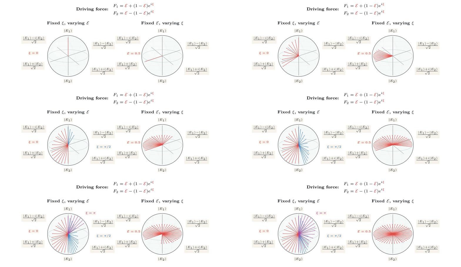
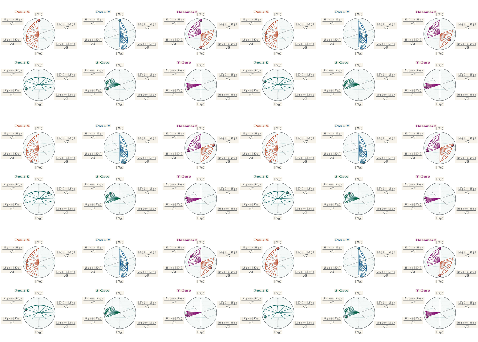
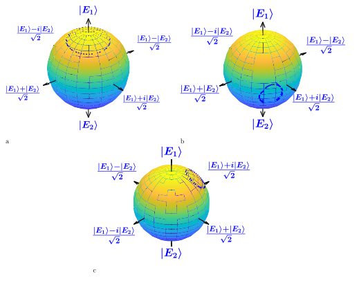
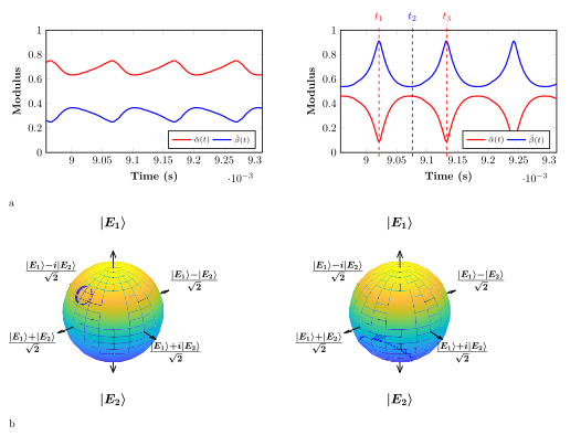
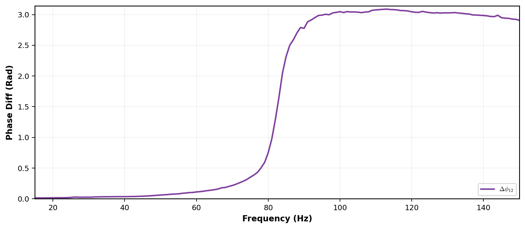
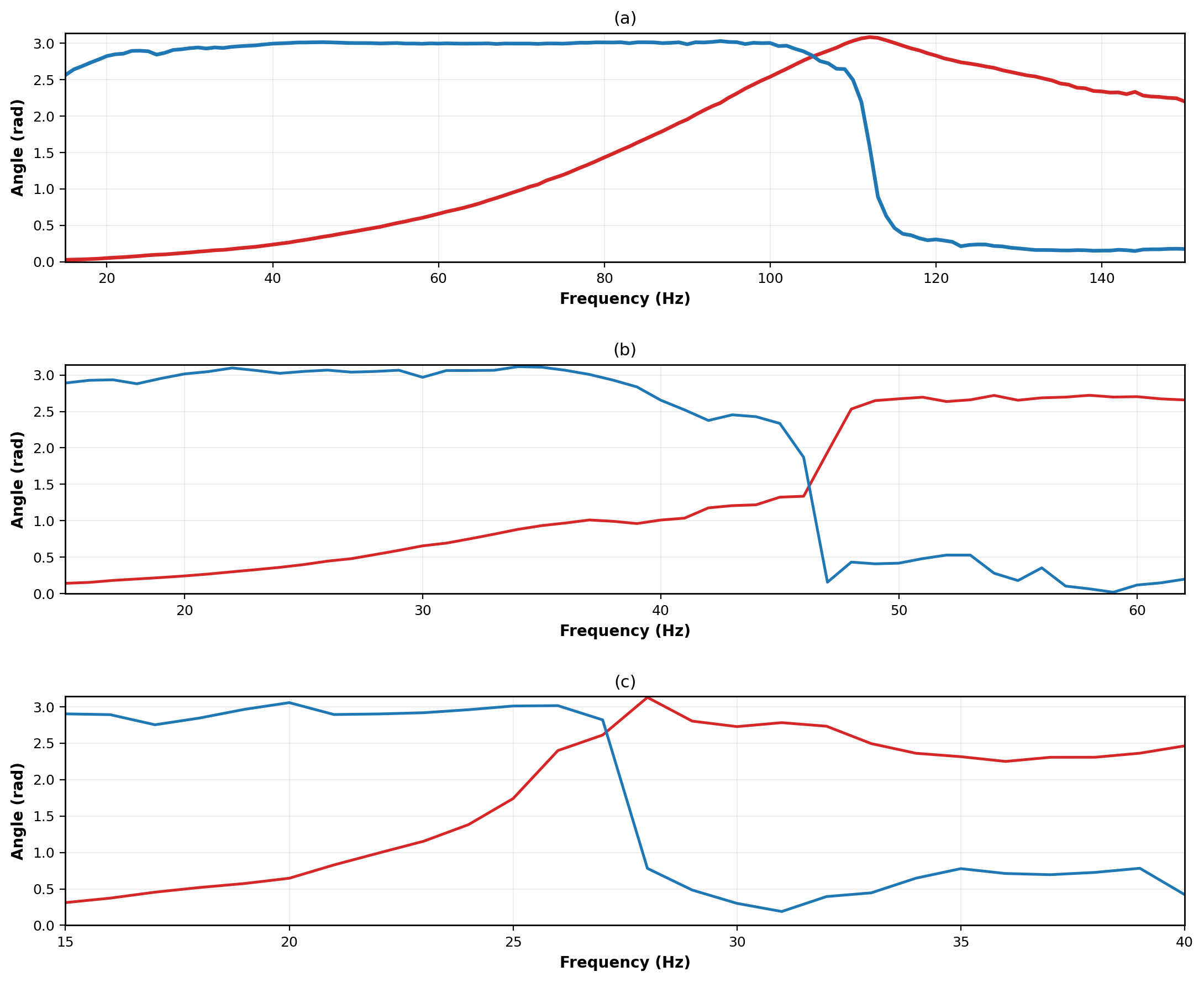
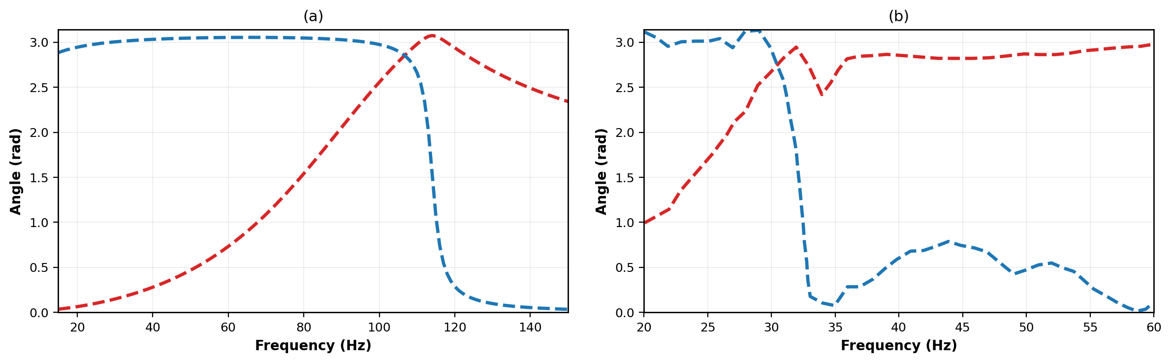
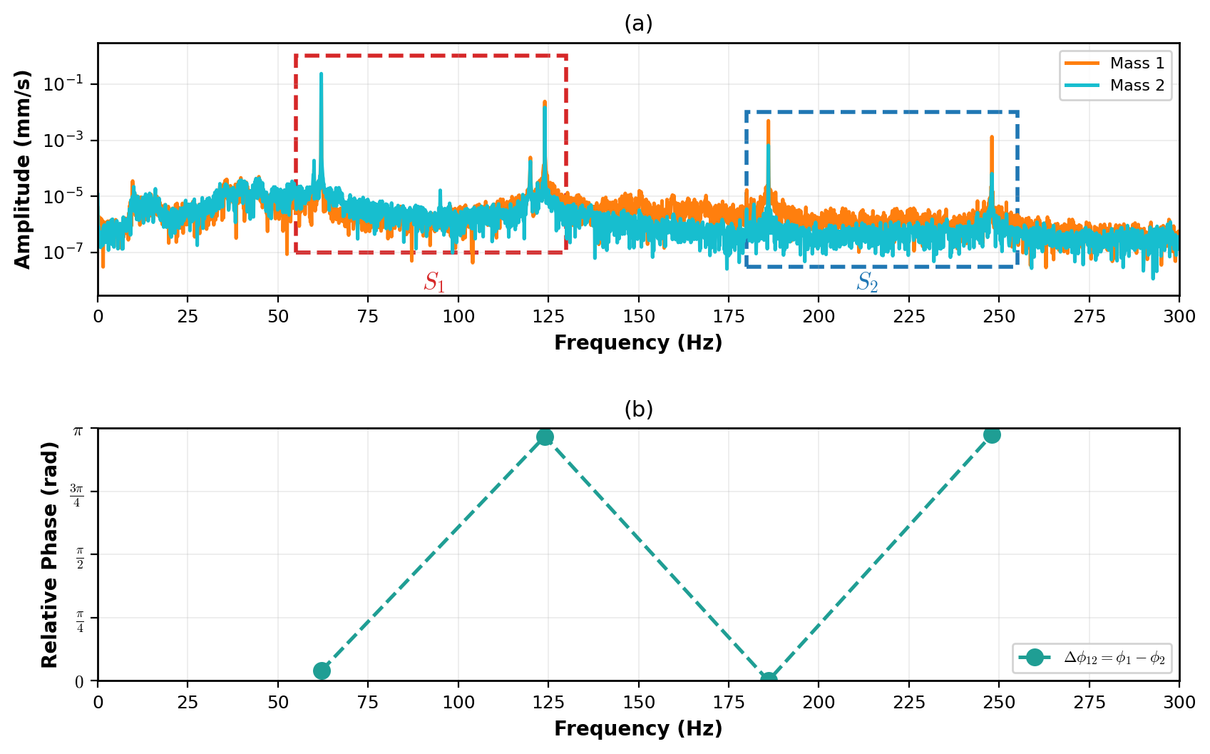
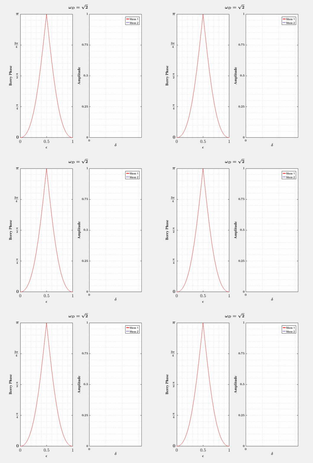
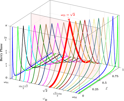
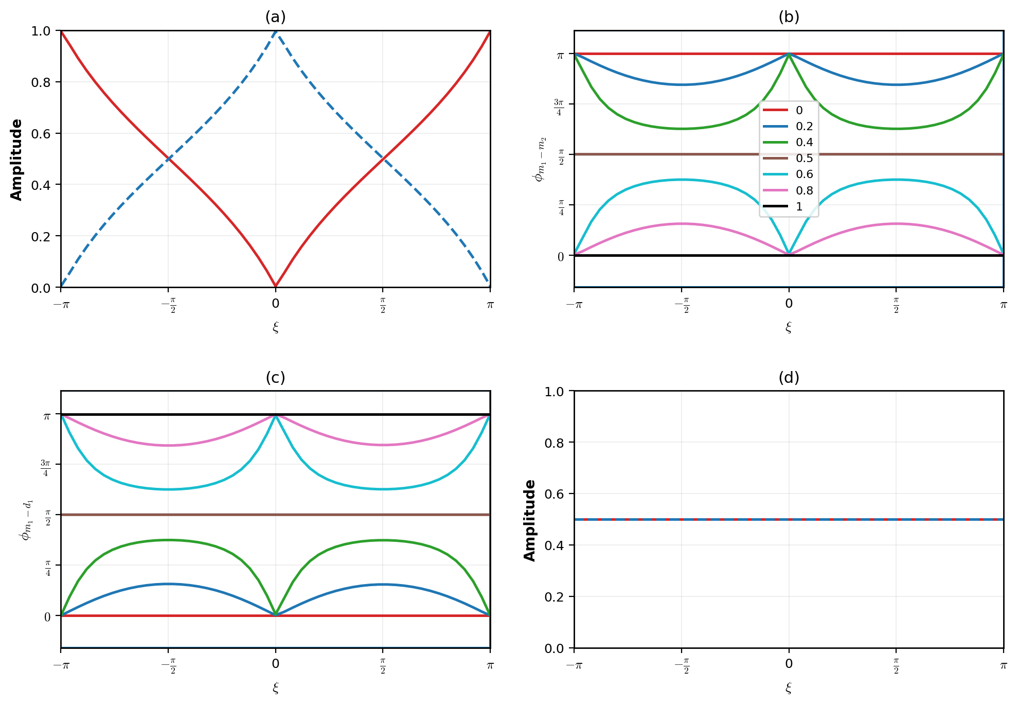
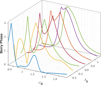
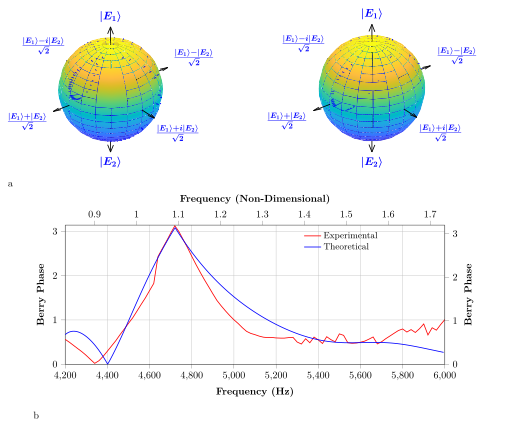
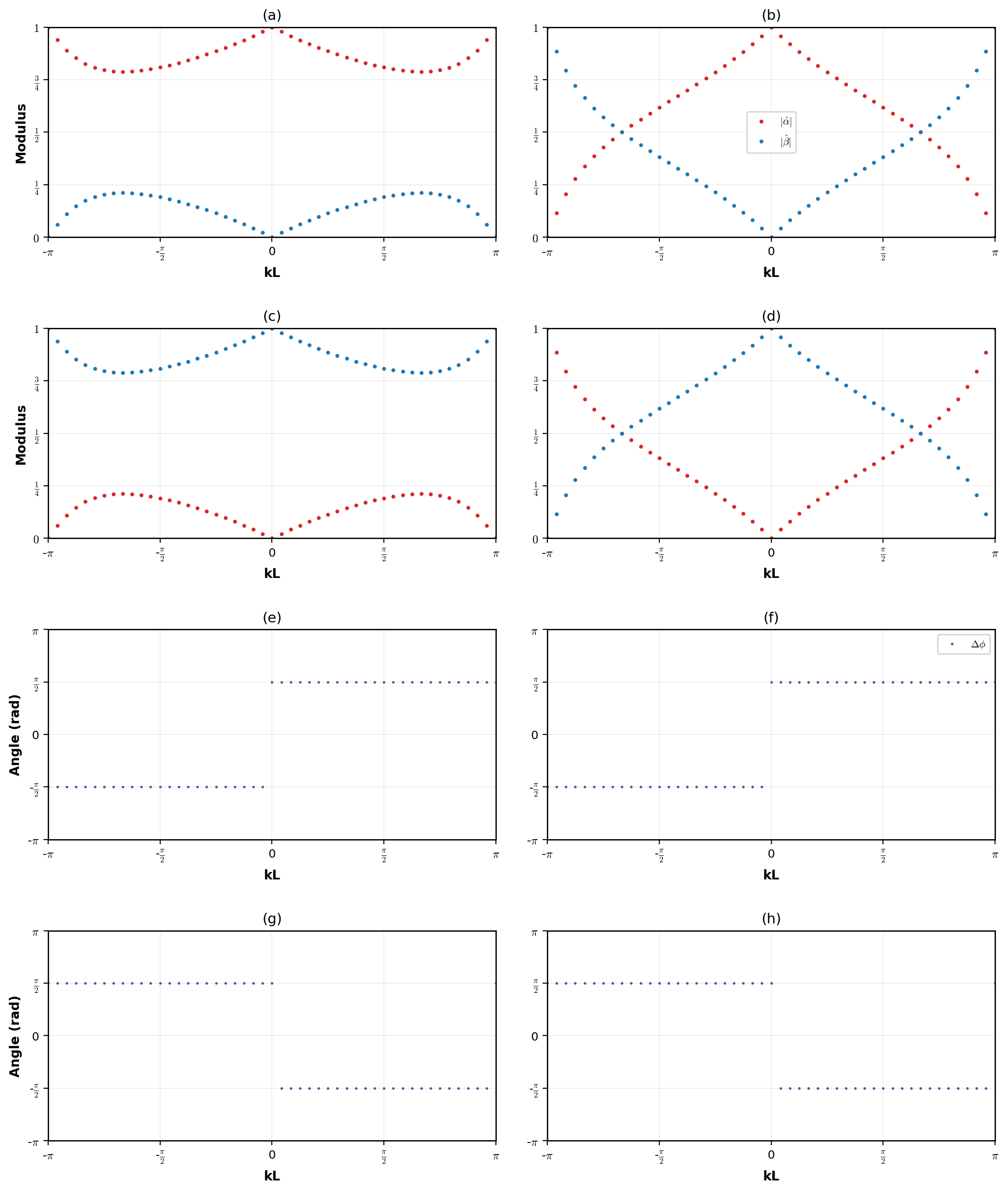
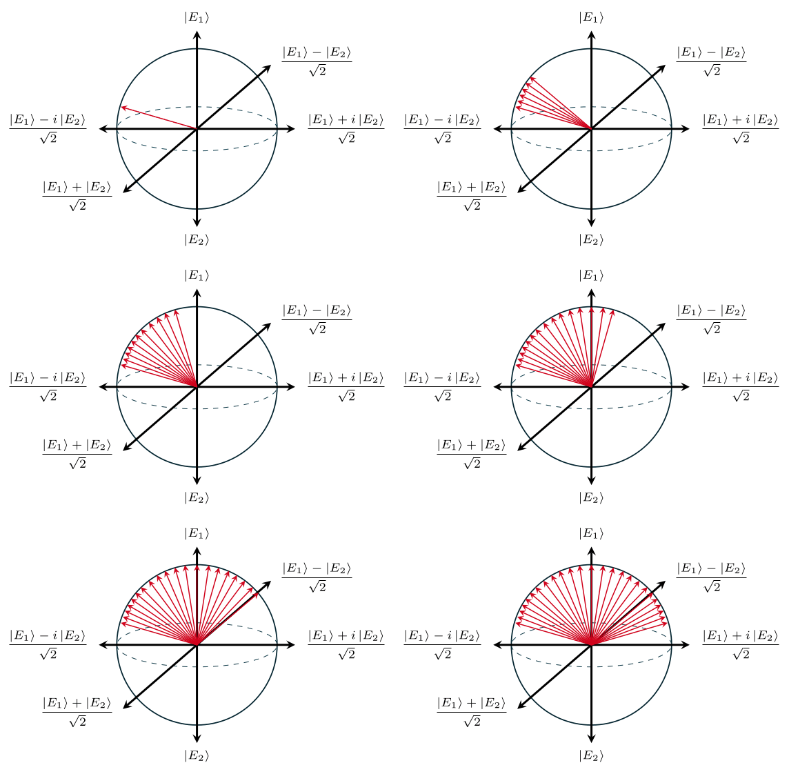
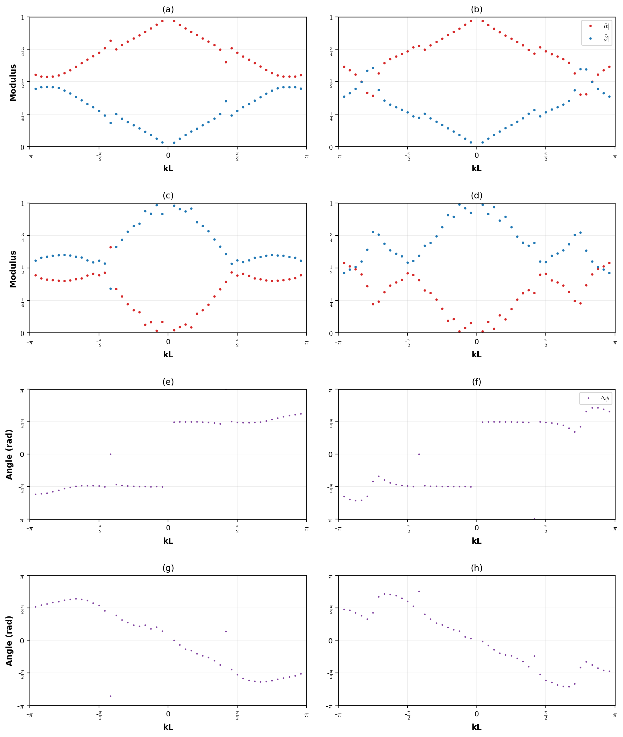
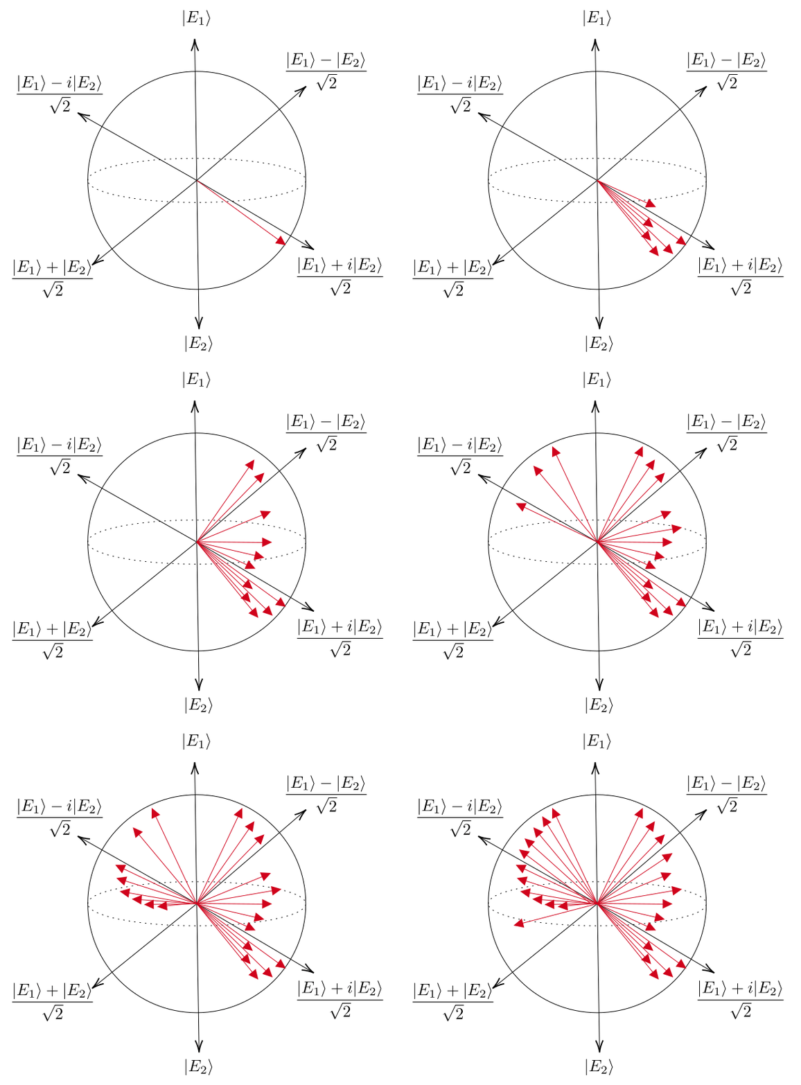
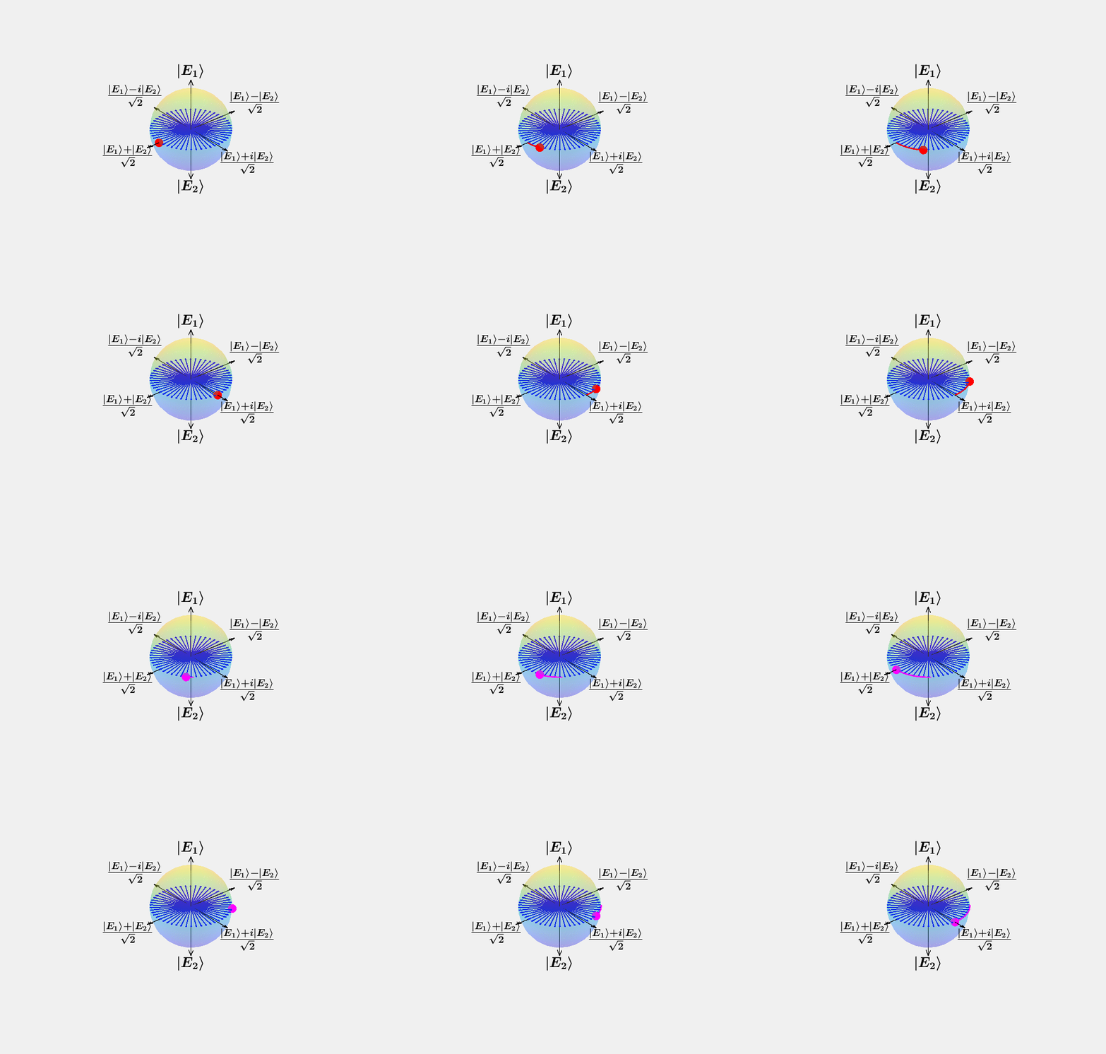
Figure 17 summarizes the analytical prediction of the Bloch-state evolution for the first and second elastic bits. The zeroth-order solution (\(\epsilon^0\)) in Fig. 17 yields the time-independent coefficients of Bit 1 and reproduces the key features of the experimental Bloch trajectory shown in Fig. 16a, including the continuous sweep of the polar angle \(\theta(\omega_d)\) and the pronounced jump in the azimuthal angle \(\phi(\omega_d)\) obtained from Eq. (70). Introducing viscous damping \(\eta\) into the analytical model smooths the otherwise abrupt phase transition and produces intermediate \(\theta\) values, thereby capturing the rounded behavior observed experimentally. Increasing \(\eta\) gradually suppresses the magnitude of the \(\varphi\) jump, consistent with the experimental trend.

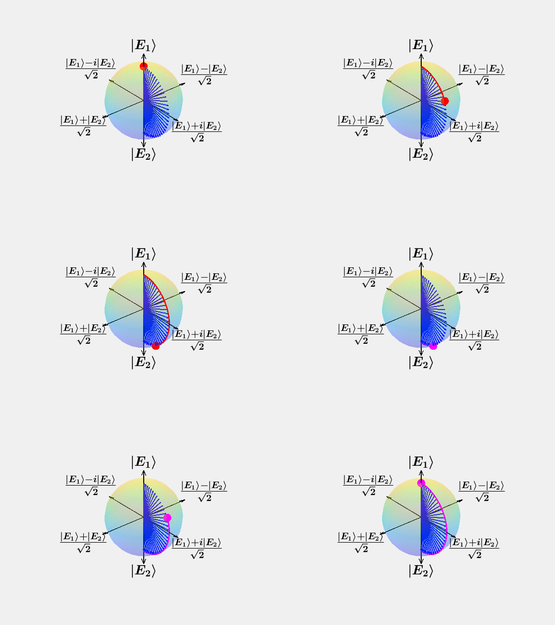
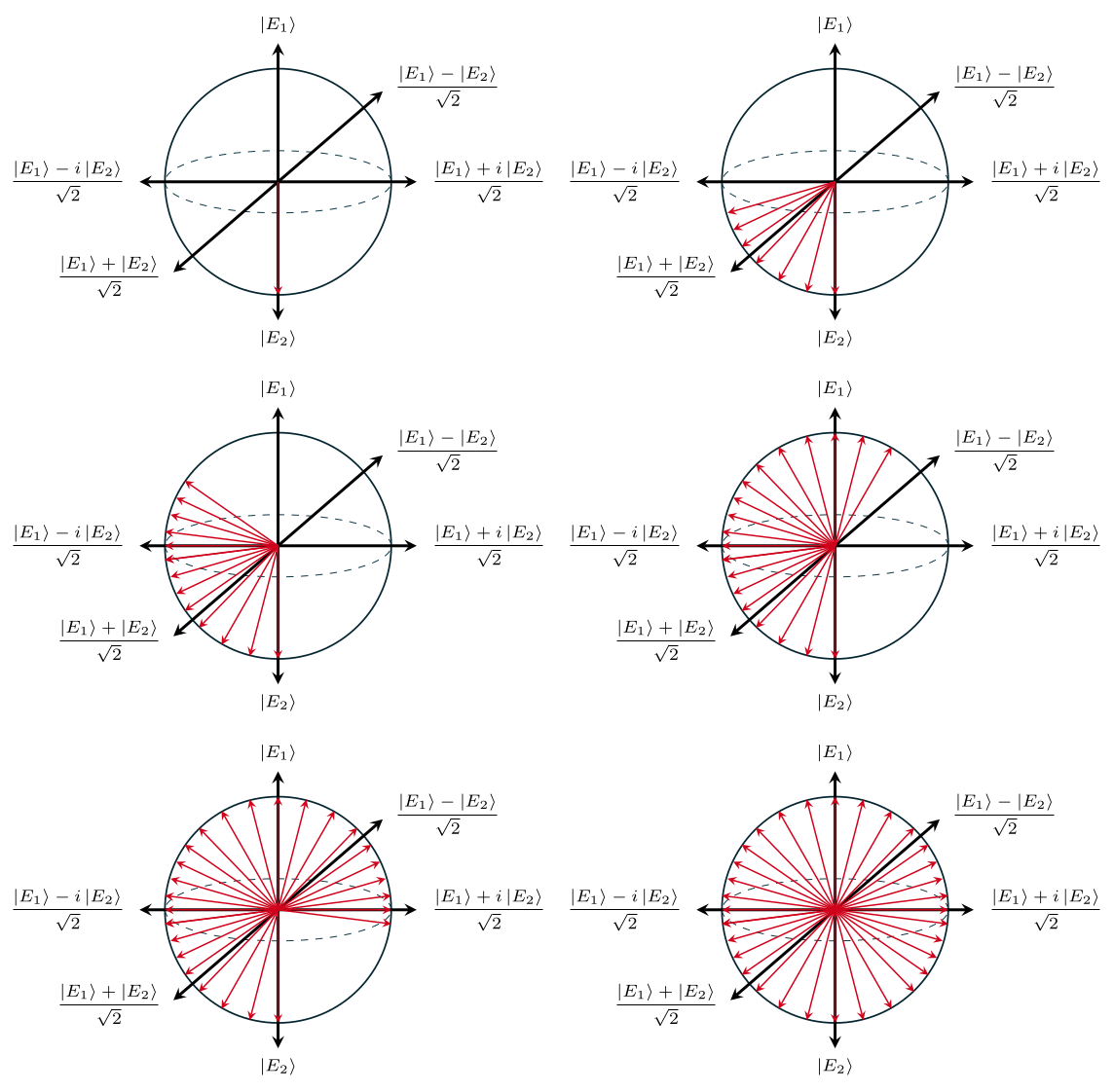
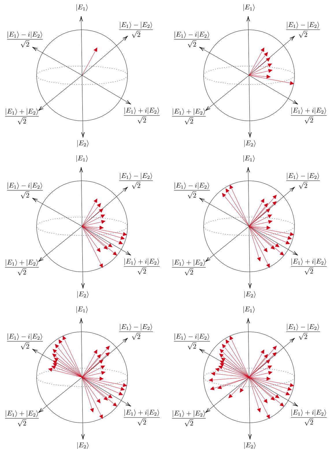
The first-order solution (\(\epsilon^1\)) generates the Bloch states for Bit 2 and yields the theoretical \(\theta(2\omega_d)\) and \(\varphi(2\omega_d)\) curves presented in Fig. 17 and Eq. (72). These curves qualitatively match the characteristic variations observed in the second-harmonic measurements of Fig. 16b, where the nonlinear response introduces additional structure and distortion in both angular trajectories. Although the analytical expressions assume idealized stiffness and simplified nonlinear contributions, the overall frequency-dependent evolution of \(\theta\) and \(\varphi\) agrees well with the experimentally measured trends. The remaining differences arise from realistic damping, asymmetric tension–compression behavior, and material-specific properties of the conical spring, all of which influence the exact shape and sharpness of the angular transitions.

The ability to freeze the internal phase while sweeping the state adiabatically is crucial for memory-type operations: information is written by selecting a point on the Bloch sphere with \(\omega_d\). It remains stable until \(\omega_d\) is changed. Hence, the time-independent logical elastic bit furnishes a robust, ambient-condition analogue of the idle qubit state that underpins quantum registers.

Dynamic (Time-Varying) States of a Single Logical Elastic Bit

When the two basis coefficients in Eq. (66) are drawn from different harmonics \((m \neq n)\), the exponential factors \(e^{i \omega_m t}\) and \(e^{i \omega_n t}\) no longer cancel. The elastic bit amplitudes therefore acquire an explicit time dependence, \(\tilde{\psi}_0(t), \tilde{\psi}_1(t) \rightarrow \tilde{\psi}_0^{(m,n)}(t), \tilde{\psi}_1^{(m,n)}(t)\), and the corresponding Bloch sphere angles evolve as

Let

So,

In this equation,

And

So,

where in the last step we used \(\cos\alpha\cos\beta+\sin\alpha\sin\beta=\cos(\alpha-\beta)\).

Which leads to,

The azimuthal angle \(\tilde{\varphi}(t)\) is formulated as

Let

with

Then

Let (\alpha=\phi_1^m+\omega_m t) and (\beta=\phi_2^n+\omega_n t), and define (a_1=|C_1^m|\sin\alpha,; a_2=|C_2^n|\sin\beta,; c_1=|C_1^m|\cos\alpha,; c_2=|C_2^n|\cos\beta.) Then

and

Moreover,

so

Therefore,

since (\sin(\beta-\alpha)=-\sin!\big[(\phi_1^m-\phi_2^n)+(\omega_m-\omega_n)t\big]). By the identity (\tan^{-1} x-\tan^{-1} y=\tan^{-1}!\big(\tfrac{x-y}{1+xy}\big)), this yields the compact form used for (\tilde{\varphi}(t)).

So,

where we used \(\sin u\cos v-\sin v\cos u=\sin(u-v)\).

And,

where the last step follows only after combining with the corresponding \(\sin^2\) terms when evaluating ( 1+xy=\dfrac{|C_1^m|^2-|C_2^n|^2}{CD} ) (cf. previous step showing (AB+CD=|C_1^m|^2-|C_2^n|^2)).

Therefore, the azimuthal angle becomes

Bloch-Sphere Precession

Equation (73) and (74) reveals that the detuning \(\Delta\omega_{mn} = |\omega_m - \omega_n|\) acts as the intrinsic precession rate of the Bloch vector: larger detuning produces faster cycles, while equal frequencies (\(\Delta\omega_{mn} = 0\)) retrieve the static states of Sec. 6.7. Geometrically, the polar angle \(\tilde{\theta}_{(m,n)}(t)\) encodes the instantaneous amplitude ratio of the in-phase \(\ket{E_1}\) and out-of-phase \(\ket{E_2}\) eigenmodes, while the azimuthal angle \(\tilde{\varphi}_{(m,n)}(t)\) captures their relative phase, exactly mirroring the qubit representation on a Bloch sphere, where the poles correspond to \(\ket{0}\) and \(\ket{1}\) states. Any other point denotes a classical superposition, and its deterministic precession under detuning closely parallels Rabi oscillations in quantum two-level systems [Cohen-Tannoudji et al., 1977].

Trajectory Engineering via Harmonic Pairing

Figure 3 plots representative trajectories \(\big(\tilde{\theta}_{(m,n)}(t),\, \tilde{\varphi}_{(m,n)}(t)\big)\) for two logical elastic bits formed by the harmonic pairs \((\omega_2,\, \omega_1)\) and \((\omega_5,\, \omega_4)\). The beating between the chosen frequencies modulates the envelope of the two-component superposition, i.e., the complex coefficients \(\big(\tilde{\psi}_0,\, \tilde{\psi}_1\big)\) in Eq. (66), with period \(T_{mn} = 2\pi / |\Delta\omega_{mn}|\), producing closed latitude- or longitude-like loops whose size and orientation are governed by the amplitude ratio \(|C_1^m| / |C_2^n|\) and phase offset \(\Delta\varphi_{mn}\).

This periodicity is essential for the calculation of the Berry phase, a topological quantity that characterizes the evolution of the state vector over time. Further, in the \((\omega_2,\, \omega_1)\) case, the polar deviation is minimal, confining the path near a line of longitude; by contrast, the \((\omega_5,\, \omega_4)\) pair sweeps a wide band across latitudes, demonstrating the tunability of state-space coverage. Because time itself parametrizes these paths, one can map any desired rotation simply by waiting the appropriate interval, without altering external drive settings.

Figure. Detuning-driven Bloch-sphere precession enables passive gate-like rotations. Time traces of \(\tilde{\theta}(t)\) and \(\tilde{\varphi}(t)\) for two logical elastic bits constructed from harmonic pairs with detuning \(\Delta\omega_{mn}=|\omega_m-\omega_n|\) illustrate deterministic, unitary evolution. Detuning \(\Delta\omega_{12}\) (pairing \(\omega_2\) and \(\omega_1\)) confines the Bloch vector to a narrow longitudinal loop of period \(T_{21}=2\pi/|\Delta\omega_{12}|\), emulating a slow \(Z\)-rotation useful for memory operations. Detuning \(\Delta\omega_{54}\) (pairing \(\omega_5\) and \(\omega_4\)) drives a wide latitude sweep that spans larger \(\tilde{\theta}\), accomplishing a full Pauli-\(X\)-like bit-flip.

Pauli-X (bit-flip).

For the frequency pair \((\omega_5,\,\omega_4)\), the state at \(t_1=9.8~\mathrm{s}\) is

Waiting a further \(\Delta t \simeq 0.04~\mathrm{s} = t_2 - t_1\) advances the phase by \((\omega_5 - \omega_4)\Delta t \approx \pi\), swapping the amplitudes exactly as a Pauli-\(X\) matrix would:

Hadamard Rotation.

Using the same pair \((\omega_5,\,\omega_4)\) and the state at \(t_1=9.8~\mathrm{s}\), advancing by \(\Delta t \simeq 0.02~\mathrm{s}\) yields

reproducing a Hadamard gate without external intervention.

These examples highlight a key advantage of the logical elastic-bit platform: time itself acts as the gate clock. By selecting suitable harmonic pairs and waiting for the appropriate beat period, single-bit rotations can, in principle, be achieved. No additional actuation, feedback, or cryogenic environment is required, only the nonlinear spectrum of the conical-spring oscillator.

Points on the Bloch sphere can be set by choosing the amplitude ratio and phase difference at a fixed drive frequency, where the pairing remains time-independent. By then switching to a detuned pairing, the required gate rotation is achieved, allowing gates to operate on arbitrary input states.

Fourier Harmonics of Mass-Conical Spring Model

The experimental system consists of two point masses coupled in series by a combination of linear and conical springs, with Mass 1 attached to an electrodynamic shaker through the linear spring and Mass 2 connected to Mass 1 via the conical spring. The graded geometry of the conical element produces an amplitude-dependent axial stiffness that is softer in tension than in compression, introducing a controlled nonlinearity without the need for additional hardware. The system is driven by a harmonic excitation at \(62\,Hz\) with a driving amplitude of \(60\,V_{p-p}\), and the steady-state out-of-plane velocities of both masses are measured using a scanning laser Doppler vibrometer. This non-contact measurement avoids mass-loading effects and ensures accurate capture of both amplitude and phase relationships across the response spectrum. Figure 19 shows the corresponding frequency response, where the top panel displays the Fourier coefficients \(|C_i|\) of the two masses on a logarithmic scale, highlighting the resonance peaks, while the bottom panel shows the absolute phase evolution as a function of frequency.

Figure. Frequency response of the two-mass system under harmonic excitation at a driving frequency of \(62\mathrm{Hz}\) with a driving amplitude of \(60\,V_{p-p}\). (19a): The Fourier magnitudes \(|C_i|\) of Mass 1 and Mass 2, highlighting resonance peaks. (19b): The corresponding relative phase between the masses with frequency. Dashed boxes indicate selected spectral regions \(S_1\) and \(S_2\).

Figure 19 summarizes the frequency-domain response of the two-mass–conical spring system under harmonic driving, showing both the spectral amplitudes and the corresponding phases that characterize the underlying modal dynamics. The top panel presents the Fast-Fourier transforms (FFTs) of the steady-state velocity signals of Mass 1 and Mass 2. A hierarchy of peaks \(|C_j^n|,\; j=1,2\), appears at harmonic orders \(n\) of the driving frequency \(\omega_n=n\omega_d\) with \(n\in\mathbb{N}\). The presence of these higher harmonics reflects the nonlinear restoring force: as the conical spring coils progressively engage under compression, the effective stiffness increases with displacement, producing spectral content beyond the fundamental. The bottom panel shows the corresponding absolute phases \(\phi_j^n,\; j=1,2\), referenced to the shaker clock as a common time origin. From these data, the phase difference \(\Delta\phi_{12}^n = \phi_1^n - \phi_2^n\) can be used to identify modal character. At the fundamental \(n=1\), the masses move nearly in-phase (\(\Delta\phi_{12}^1 \approx 0\)), consistent with the linearized in-phase eigenmode \(\ket{E_1}=\tfrac{1}{\sqrt{2}}\begin{pmatrix}1\\1\end{pmatrix}\). At the second harmonic \(n=2\), the phase difference approaches \(\pi\), corresponding to the out-of-phase eigenmode \(\ket{E_2}=\tfrac{1}{\sqrt{2}}\begin{pmatrix}1\\-1\end{pmatrix}\). For higher harmonics \(n>2\), \(\Delta\phi_{12}^n\) deviates from \(0\) or \(\pi\), indicating that the response corresponds to controlled superpositions of \(\ket{E_1}\) and \(\ket{E_2}\) generated by nonlinear mixing.

Two Logical Elastic Bits with Time-Variant Complex Coefficients

We construct two logical elastic bits by projecting the driven two-mass, conical-spring system’s velocity field onto the orthonormal pair of linear eigenmodes, \(\ket{E_1}\) and \(\ket{E_2}\), at selected characteristic frequencies and then forming tensor-product states across those Fourier components [Mahmood et al., 2025]. This procedure generates a four-level, quantum-like state whose complex amplitudes evolve in time under steady excitation. Although nonlinear normal modes lack strict orthogonality, the in-phase and out-of-phase linear eigenmodes supply a complete orthonormal basis at each frequency, ensuring that the measured or simulated multi-harmonic response can be decomposed unambiguously. The resulting coefficients, denoted \(\tilde{\psi}_{00}\), \(\tilde{\psi}_{01}\), \(\tilde{\psi}_{10}\), and \(\tilde{\psi}_{11}\), inherit explicit temporal factors such as \(e^{i\omega t}\), which encode deterministic evolution without auxiliary control. In this way, the coupled oscillator defines a mechanical analogue of a two-bit Hilbert space, where the instantaneous state vector \([\tilde{\psi}_{00}(t), \tilde{\psi}_{01}(t), \tilde{\psi}_{10}(t), \tilde{\psi}_{11}(t)]^{T}\) represents the spectral content of the response.

Equation (75) shows explicitly how the Fourier amplitudes map onto the tensor-product basis, with each term corresponding to a distinct combination of eigenstates. The first pair of eigenvectors, \(\ket{E_1^1}\) and \(\ket{E_2^1}\), span a two-dimensional Hilbert space \(\mathcal{H}_1\), while the second pair, \(\ket{E_1^1}\) and \(\ket{E_2^1}\), span another, \(\mathcal{H}_2\). Taken together, these define the four-dimensional composite space \(\mathcal{H}_{\varepsilon} = \mathcal{H}_1 \otimes \mathcal{H}_2\). Here, the symbol \(\otimes\) denotes the tensor product, which combines basis states of the two subsystems into joint states of the composite system. For example, \(\ket{E_1^1} \otimes \ket{E_2^2}\) represents the state in which subsystem \(S_1\) is in eigenstate \(\ket{E_1^1}\) while subsystem \(S_2\) is simultaneously in eigenstate \(\ket{E_2^2}\). In this way, the tensor-product basis spans all possible joint configurations of the two e-bits, allowing the dynamics of the coupled system to be described as a superposition of these product states. Within this framework, the displacement field at each characteristic frequency can be represented as a normalized state vector in Dirac notation, with time-dependent coefficients \(\tilde{\psi}_{ij}(t)\) encoding both amplitude and phase. This formulation highlights that the nonlinear oscillator admits a structured composite state space, in which the system’s response can be expressed as time-dependent superpositions of tensor-product basis states.

An e-bit is a two-level subsystem defined by the orthonormal eigenmode pair of a selected spectral segment (e.g., \(\ket{E_{1}^{1}},\ket{E_{2}^{1}}\) for \(S_1\) and \(\ket{E_{1}^{2}},\ket{E_{2}^{2}}\) for \(S_2\)). At a chosen characteristic frequency, projecting the measured response onto this basis yields two complex Fourier coefficients: their magnitudes are the measured harmonic amplitudes \((|C_i^{j}|)\) and their arguments are the corresponding phases \((\phi_i^{j})\) referenced to the drive. After normalization, these amplitudes and phases directly specify the state. For two e-bits, the experimentally extracted coefficients populate the tensor-product basis \(\mathcal{H}_{\varepsilon}=\mathcal{H}_{1}\otimes\mathcal{H}_{2}\), so \(\tilde{\psi}_{00}(t),\tilde{\psi}_{01}(t),\tilde{\psi}_{10}(t),\tilde{\psi}_{11}(t)\) are the measurable complex weights of \(\ket{E_{i}^{1}}\otimes\ket{E_{j}^{2}}\). This tensor-product description does not assume two physically isolated oscillators: all components originate from the same nonlinear device, and nonlinear coupling appears as generally non-separable coefficient patterns, while distinct segments remain separable in the frequency-domain representation under the chosen resolution. Practical readout therefore consists of extracting \(\tilde{\psi}_{ij}(t)\) at the selected harmonics, normalizing, and assigning the logical state from the weights \(|\tilde{\psi}_{ij}|^{2}\) and relative phases \(\arg(\tilde{\psi}_{ij})\). In practice, the validity of treating segments as separate readout channels is supported by the experimentally observed spectral isolation and repeatability of the extracted complex coefficients, i.e., negligible cross-band leakage within the chosen bandwidth and stable phase references across repeated acquisitions.

Multi-Segment Spectral Embedding and Intrinsic Gate-Like Evolution

To capture the temporal richness of the nonlinear response, the construction can be extended beyond a single spectral segmentation. Instead of restricting to one pair of Fourier components, we combine multiple spectral segments, each associated with a distinct harmonic order. This approach preserves the time dependence of the amplitudes while embedding the response into the same tensor-product basis, thereby allowing the elastic state to be expressed as a superposition across several frequency channels. The formal structure of this multi-segment decomposition is summarized in Eq. (75).

Equation (76) generalizes the two-bit elastic state by incorporating multiple Fourier components from distinct spectral segments. Each summand corresponds to a particular harmonic order \(n\), with coefficients \(\tilde\psi_{ij,n}(t)\) that evolve in time according to the nonlinear dynamics. By summing up these contributions, we obtain effective amplitudes \(\tilde{\psi}_{ij}(t)\) that retain explicit time dependence and encode modal mixing across harmonics. This construction emphasizes that the logical e-bit framework is not limited to a single pair of frequencies but can naturally integrate higher-order content while remaining embedded in the tensor-product basis. The resulting state vector, expressed as a linear combination of \(\left|E_i^{S_1}\right\rangle \otimes \left|E_j^{S_2}\right\rangle\), thus provides a compact description of the nonlinear oscillator’s spectral response, suitable for interpreting its dynamics as gate-like operations within a four-dimensional Hilbert space.

The segmentation into \(S_{1}\) and \(S_{2}\) is introduced to ensure that each e-bit is constructed from Fourier components that are both physically distinct and experimentally robust. In practice, each segment is anchored around a resolved harmonic order (or a small cluster of closely spaced harmonics) selected from the measured spectrum, and the segment boundaries are chosen so that: (i) the dominant peak(s) defining that harmonic order remain fully contained within the segment, (ii) the selected peaks do not overlap with neighboring peaks within the frequency resolution of the FFT (minimizing leakage and cross-talk between segments), and (iii) the retained harmonic content has sufficient signal-to-noise ratio for reliable phase extraction relative to the excitation reference. Under these criteria, \(S_{1}\) and \(S_{2}\) provide a consistent partition of the spectrum so that the same modal basis and tensor-product structure can be applied across multiple harmonic orders in Eq. (76). Sensitivity to segmentation is mainly determined by the harmonic peaks that define each segment. Small shifts in the boundaries are usually benign as long as they still contain the same dominant peaks, leading only to minor quantitative changes through leakage and weighting. By contrast, switching harmonic order or replacing a peak with a neighbor changes \(\tilde\psi_{ij,n}(t)\), since the nonlinear oscillator couples different harmonics with different strength and phase. Consequently, the qualitative multi-bit structure and the gate-like interpretation remain stable for any segmentation that preserves the peak-anchored, non-overlapping, high-SNR selection, while the detailed coefficient trajectories reflect the specific harmonic content chosen for the state embedding.

Collecting these contributions into a single object clarifies both the basis and the time dependence of the amplitudes; we therefore define the composite two-bit state as,

Here, the indices \(i,j,p,q\) label the harmonic components of the nonlinear mass responses, as identified in Fig. 20, and can be selected from either fundamental or higher-order Fourier content depending on the spectral resolution of interest. The subscripts \(m\) and \(n\) denote the two physical masses of the oscillator. Different indices choices correspond to different embeddings/bases and can lead to different effective operators, but once the indices are fixed the resulting state and the associated gate-like mapping are uniquely determined by the measured evolution. This flexibility therefore does not imply universality by relabeling; the achievable operation set is still constrained by the intrinsic dynamics and available control parameters. This formulation emphasizes that the choice of harmonic indices is flexible, enabling different frequency components to be combined within a single basis representation. Consequently, the total displacement field is expressed as an expansion in the product Hilbert space \(\mathcal{H}_{\varepsilon}\), with time-dependent complex coefficients \(\tilde{\psi}_{ij}(t)\) that encode both the modal structure and the nonlinear mixing across harmonics. After normalization of Eq. (77), the state is a unit vector in a complex, four-dimensional Hilbert space spanned by the orthonormal product \(\left[\left|E_1^{S_1}\right\rangle \otimes \left|E_1^{S_2}\right\rangle, \left|E_1^{S_1}\right\rangle \otimes \left|E_2^{S_2}\right\rangle, \left|E_2^{S_1}\right\rangle \otimes \left|E_1^{S_2}\right\rangle, \left|E_2^{S_1}\right\rangle \otimes \left|E_2^{S_2}\right\rangle \right]\). The coefficients \(\tilde{\psi}_{ij}(t)\) encode the instantaneous modal content, both amplitude and phase, and their joint structure determines separability: a necessary condition for a non-separable (classically entangled) state is \(\tilde{\psi}_{00}\tilde{\psi}_{11} \neq \tilde{\psi}_{01}\tilde{\psi}_{10}\) [Nielsen and Chuang, 2000]. Importantly, Eq. (77) distinguishes linear from nonlinear operation: in a linear elastic system, where no modal mixing occurs, a single harmonic suffices and \(\tilde{\psi}_{ij}\) are time-independent [Mahmood and Hasan, 2025]; in the nonlinear regime studied here, higher-order content drives explicit time dependence in \(\tilde{\psi}_{ij}\), enabling controlled evolution of the superposed product states within the same fixed basis.

Figure. Temporal evolution of the joint two e-bits state coefficients for two Fourier-segment selections. The upper panels show the real parts and the lower panels the imaginary parts of \(\tilde{\psi}_{00}(t)\), \(\tilde{\psi}_{01}(t)\) , \(\tilde{\psi}_{10}(t)\), and \(\tilde{\psi}_{11}(t)\). Vertical dashed lines indicate time instants \(t_1\) (red) and \(t_2\) (blue). (20a) Segment choice \([C_1^2; C_2^1; C_1^1; C_2^2]\) leads to time-dependent variation in the relative amplitudes and phases of the four joint state coefficients. (20b) Segment choice \([C_1^1; C_2^2; C_1^2; C_2^1]\) produces a distinct temporal pattern of relative amplitudes and phase evolution.

Figure 20 illustrates the temporal evolution of the two-bit state coefficients under two representative driving conditions. In both cases, the upper panels show the real parts of \(\tilde{\psi}_{00}(t)\), \(\tilde{\psi}_{01}(t)\), \(\tilde{\psi}_{10}(t)\), and \(\tilde{\psi}_{11}(t)\), while the lower panels display their imaginary parts. Each coefficient follows an oscillatory trajectory, with relative phase shifts and amplitude modulations that reflect the nonlinear mixing of Fourier components. Panel (20a) corresponds to the segment combination \([C_1^1;C_2^1;C_1^2;C_2^2]\), while panel (20b) corresponds to \([C_1^1;C_2^2;C_1^2;C_2^1]\), showing how different selections of harmonic pairs alter the relative evolution of the coefficients. These results confirm that the distribution of weight among the tensor-product states is not fixed but depends directly on how the Fourier spectrum is partitioned into segments. In this way, the figure highlights both the persistence of the superposition in time and its tunability, demonstrating that the logical elastic states can be shaped by the specific choice of spectral components extracted from the nonlinear response.

As seen in Fig. 20, the passage of time effectively tunes the superposition generated by the Fourier-mode eigenstates of the logical elastic bit. Thus, the temporal dynamics act as an intrinsic unitary transformation, mapping one state to another without the need for external modulation. For instance, the system state at \(t_1\) can be written as \(\lvert \psi(t_1) \rangle\), which evolves naturally into \(\lvert \psi(t_2) \rangle\) at a later time. This process is mathematically equivalent to applying a gate operation, as illustrated below:

The transformation above corresponds to a \(\pi\)-phase gate, applied uniformly to the four-dimensional state vector. Importantly, the mapping is reversible: the same operation can carry \(\tilde{\psi}(t_1)\) forward to \(\tilde{\psi}(t_2)\) or backward from \(\tilde{\psi}(t_2)\) to \(\tilde{\psi}(t_1)\). By adjusting the substitution procedure used to calculate the transformation matrix, one can obtain diagonal or off-diagonal forms, each corresponding to different gate actions at distinct times. This flexibility confirms that different effective transformations are accessible depending on the choice of time instants.

The dynamic behavior of \(\lvert \tilde{\psi}_{ij}(t)\rangle\) therefore demonstrates the system’s intrinsic capability to realize quantum-analogous gates without external feedback or active control. Gate functionality emerges directly from the nonlinear spectral structure and natural time evolution of the mechanical system. These results establish that the two-bit logical elastic system behaves analogously to quantum gates operating in a four-level Hilbert space, providing a platform for exploring classical counterparts of entanglement, gate-based operations, and even multi-bit circuit analogues using purely mechanical degrees of freedom.

Modal-State Transformation via Householder Reflection

The experimentally measured modal responses at selected time instants correspond to distinct points along a repeatable dynamical orbit of the coupled nonlinear oscillator. Because the system operates in a steady nonlinear regime, these points represent stable configurations of the whole elastic state rather than transient responses. As time evolves, the complex modal coefficients change in a correlated manner within a low-dimensional space defined by the measured amplitudes and phases. Upon selecting two distinct time instants \(t_1\) and \(t_2\), the joint e-bit state evolves from \(\ket{\tilde{\psi(t_1)}}\) to \(\ket{\tilde{\psi(t_2)}}\). This temporal evolution constitutes a physical operation that results in a change of the corresponding four-dimensional state vector in the two-bit elastic Hilbert space.

Describing this evolution in a physically meaningful way requires identifying a single linear operator that maps the complete state vector at time \(t_1\) to that at time \(t_2\). In a state-based description of information processing, such state-to-state mapping defines an operation: a gate or algorithm is specified by the transformation that converts one input state into an output state. Since the observed evolution preserves normalization and relative phase relationships, the corresponding transformation must be unitary, ensuring reversibility of the mapping. The unitary-like characterization can be verified directly from the reconstructed coefficients by tracking the norm of the instantaneous two-bit state vector \([\tilde{\psi}_{00}(t),\,\tilde{\psi}_{01}(t),\,\tilde{\psi}_{10}(t),\,\tilde{\psi}_{11}(t)]^{T}\) over the same steady-state window used for the state-to-state mapping. Specifically, at each time instant the quantity \(|\tilde\psi_{00}(t)|^2+|\tilde\psi_{01}(t)|^2+|\tilde\psi_{10}(t)|^2+|\tilde\psi_{11}(t)|^2\) is evaluated after applying the same normalization procedure used to form the state representation. In an ideal lossless and perfectly phase-resolved case this value remains unity; experimentally, small departures from unity quantify the combined effect of damping-driven amplitude modulation and measurement limitations such as finite FFT resolution/leakage and phase jitter in low-SNR harmonic components. Reporting the time variation of this norm (and its deviation from unity) therefore provides a quantitative basis for describing the evolution as unitary-like in the normalized coefficient space, while clearly identifying non-idealities attributable to dissipation and noise.

The Householder reflection provides an exact and minimal construction of this unitary transformation. Here, the operator is not introduced as an additional physical element acting on the oscillator, but as a compact representation of the experimentally observed state-to-state evolution in the normalized coefficient space. The nonlinear system evolves autonomously under steady excitation, and the measured multi-bit state vectors at two instants \(t_1\) and \(t_2\) provide the input–output pair for identifying an effective mapping \(U(t_2,t_1)\). The Householder construction is employed because it yields an exact unitary map that takes one normalized measured state to the other while preserving relative phase structure; it should therefore be interpreted as an effective propagator extracted from data rather than an externally imposed control gate. Different choices of \((t_1,t_2)\) can yield different effective mappings because they summarize different portions of the same intrinsic dynamical orbit, but in each case the operator is determined uniquely by the measured states within the selected Hilbert-space representation. Given two normalized experimental state vectors \(\ket{\tilde{\psi}(t_1)}\) and \(\ket{\tilde{\psi}(t_2)}\), it yields a Hermitian and unitary operator that maps one state onto the other while preserving their collective amplitude-phase structure [Householder, 1958]. In this sense, the Householder operator represents the effective gate enacted by the intrinsic nonlinear time evolution, directly linking the experimentally observed modal transitions to gate-like operations within the logical e-bit framework [Co, 2013]. An analogous state-to-state mapping approach was previously used to identify nontrivial multi-bit unitary operations in nonlinear acoustic phi-bit systems, where tuning a physical control parameter resulted in a deterministic unitary transformation acting on an exponentially scaling Hilbert space [Deymier et al., 2023]. Here, time evolution plays the role of the control parameter, and the resulting \(4 \times 4\) unitary matrix captures how nonlinear elastic dynamics implement a structured operation on the joint two-bit state.

Within the tensor-product representation, the instantaneous two-bit elastic state of the coupled system resides in the composite Hilbert space \(\mathcal{H}_{\varepsilon} = \mathcal{H}_1 \otimes \mathcal{H}_2\), where each subspace \(\mathcal{H}_n\) (\(n = 1,2\)) corresponds to a distinct modal channel of the nonlinear medium, typically associated with characteristic drive frequencies. The orthonormal eigenmodes \([\ket{E_1^1}, \ket{E_2^1}]\) and \([\ket{E_1^2}, \ket{E_2^2}]\) span the local Hilbert spaces, and their tensor products form the complete modal basis

The experimentally obtained modal state vectors at different two-time instants are

where each component represents the complex amplitude of a particular modal combination.

To determine the single-step transformation that converts \(\tilde{\psi}(t_1)\) into \(\tilde{\psi}(t_2)\), the Householder reflection is constructed as

which satisfies both \(U^{\dagger} = U\) and \(U^2 = I\), confirming that it is Hermitian and unitary. These properties ensure that \(U\) performs a reversible mapping between the two measured modal states, such that

Numerically,

and applying \(U\) to \(\tilde\psi(t_1)\) reproduces \(\tilde\psi(t_2)\) up to a global phase factor, confirming the validity of the reflection. A global phase factor here means that all components of the reconstructed state acquire the same phase offset. Because the coefficients are extracted with the excitation as the phase reference, such a common offset corresponds to a uniform shift of the timing reference and leaves all relative phase relationships, and therefore the basis weights and gate identification unchanged. In the special case of a \(\pi\) shift, this appears as a sign inversion of the measured harmonic response relative to the reference, without changing any relative phases among the coefficients. The eigenvalues of \(U\) are \([-1, +1, +1, +1]\), indicating a single inverted direction and a three-dimensional invariant subspace orthogonal to it. These eigenvalues follow because \(U\) is a Householder reflection, which is unitary by construction. This unitarity applies to the normalized state-space mapping, while damping appears as imperfect normalization/state-mapping error in the measured coefficients, not as a change in the eigenvalue magnitudes of the constructed \(U\). The normalized vector \(\hat{v} = v / |v|\) defines the reflection direction in the Hilbert space, and the corresponding operator

introduces a phase inversion along \(\hat{v}\) while preserving all orthogonal components. To interpret the transformation geometrically, \(U\) can be factorized as

where \(W\) is a preparatory rotation that aligns the modal coordinate frame with the reflection hyperplane, \(R\) is the canonical reflection kernel, and \(W^{\dagger}\) restores the system to its original coordinates. This decomposition reveals that \(W\) reorients the basis according to the experimental states, \(R\) introduces the \(\pi\)-phase inversion in that aligned frame, and \(W^{\dagger}\) reverses the alignment, yielding a lossless, deterministic transformation that preserves both energy and phase coherence. The rotation operator \(W\) is obtained from the two measured states as

This ensures that \(\tilde\psi(t_1)\) is mapped onto the reflection axis in the rotated frame, where the reflection and restoration complete the overall transformation.

The canonical reflection kernel \(R\) can be expressed using minimal two-qubit gate analogues as

With

And

This form represents a reflection about the first computational basis vector and demonstrates the equivalence between modal reflections and canonical quantum operations. The complete transformation between \(\tilde\psi(t_1)\) and \(\tilde\psi(t_2)\) can therefore be written as

In this framework, \(\mathcal{H}_1\) and \(\mathcal{H}_2\) correspond to distinguish the Hilbert space of the nonlinear system, and the operator \(U\) acts as a geometric mirror in the four-dimensional modal Hilbert space, rotating the complete spectral configuration from one measured state to another through a single deterministic operation. Expressed in gate form, the same transformation decomposes into a concise sequence of modal rotations and controlled phase inversions, the mechanical counterparts of Pauli-\(X\) and controlled-\(Z\) gates. For a given measured initial and final normalized state, the Householder construction yields a unique \(U\) because it is defined by a fixed mapping rule. More generally, many unitary operators can map the same initial state to the same final state by differing only in their action on the orthogonal subspace, so a single state-to-state transition does not determine a unique space-wide operator. This ambiguity implies that the reported \(U\) should be interpreted as an effective representation of the observed evolution along the measured trajectory unless additional state transitions are used to further constrain the operator. This establishes that the nonlinear elastic network supports a fully classical analogue of two-bit logical transformations governed by deterministic, decoherence-free dynamics, thereby unifying experimentally observed modal transitions with canonical operations of quantum logic.

Time Variant Entropy of Entanglement of Logical Elastic Bit

To quantify the degree of non-separability between the two elastic bits, we calculate the entropy of entanglement, which serves as a rigorous measure of correlations embedded in the time-dependent coefficients. Starting from the composite state \(\lvert \Psi(t)\rangle = \sum_{i,j \in \{0,1\}} \tilde{\psi}_{ij}(t)\, \lvert E_i^{S_1}\rangle \otimes \lvert E_j^{S_2}\rangle\), we first construct the density matrix of the full system,

(82)\[\begin{equation} \rho(t) = \lvert \Psi(t) \rangle \langle \Psi(t)\rvert. \end{equation}\]

Since we are interested in the correlations between the two subsystems, we compute the reduced density matrix by tracing over one elastic bit, for example

(83)\[\begin{equation} \rho_{S_1}(t) = \mathrm{Tr}_{S_2}\,\rho(t), \qquad \rho_{S_2}(t) = \mathrm{Tr}_{S_1}\,\rho(t). \end{equation}\]

The entropy of entanglement is then obtained from the von Neumann entropy of the reduced state,

(84)\[\begin{equation} S_p(t) = -\,\mathrm{Tr}\big[\, \rho_{S_1}(t) \,\log \rho_{S_1}(t)\,\big] = -\,\mathrm{Tr}\big[\, \rho_{S_2}(t) \,\log \rho_{S_2}(t)\,\big]. \end{equation}\]

For a pure bipartite state this entropy is uniquely defined and quantifies the extent to which the system cannot be factorized into independent single-bit contributions. Explicitly, if \(\lambda_1(t)\) and \(\lambda_2(t)\) denote the nonzero eigenvalues of the reduced density matrix, then the entropy of entanglement becomes

(85)\[\begin{equation} S_p(t) = - \sum_{k=1}^{2} \lambda_k(t)\,\log \lambda_k(t). \end{equation}\]

In the separable limit, one eigenvalue equals unity and the other vanishes, leading to \(S_p(t)=0\). In the maximally non-separable limit, both eigenvalues converge to \(1/2\), and the entropy reaches \(S_p(t)=\log 2\). Thus, the temporal profile \(S_p(t)\) reveals how nonlinear mode mixing and Fourier-segment contributions dynamically generate and suppress correlations between the elastic bits. In this framework, separability corresponds to vanishing entropy, while non-separability is signaled by finite entropy, with the magnitude encoding the strength of the effective entanglement.

Figure. Time-dependent entropy of entanglement for two Fourier-segment selections. (a) For \([C_1^1;C_2^1;C_1^2;C_2^2]\), the entropy remains at \(S_p(t)\approx 0\), consistent with a separable state where the two subsystems evolve independently. (b) For \([C_1^1;C_2^2;C_1^2;C_2^1]\), the entropy stays finite at \(S_p(t)\approx 0.6\) with small oscillations, indicating persistent non-separability and sustained correlations between the elastic bits. The contrast between (a) and (b) highlights how the choice of Fourier-segment partitioning directly controls whether the system exhibits separable or classically entangled behavior.

The entropy results in Fig. 21 can be directly correlated with the coefficient trajectories shown previously in Fig. 20. In panel (21a), the real and imaginary parts of \(\tilde{\psi}_{00}(t)\), \(\tilde{\psi}_{01}(t)\), \(\tilde{\psi}_{10}(t)\), and \(\tilde{\psi}_{11}(t)\) evolved in a manner that preserved strong proportionality between products of coefficients, consistent with the separability condition \(\tilde{\psi}_{00}\tilde{\psi}_{11}=\tilde{\psi}_{01}\tilde{\psi}_{10}\). This fixed relational pattern between the traces explains why the entropy remains pinned at zero: the dynamics involve only redistribution within each bit, and no correlations arise between subsystems. By contrast, in panel (21b) of Fig. 20, the four coefficients displayed distinct amplitudes, phase shifts, and repeated crossings, clear signatures of non-separability. These departures from proportional evolution feed directly into the reduced density matrix, producing two nontrivial eigenvalues and hence a finite entropy in Fig. 21b. The nearly constant value of \(S_p(t)/\log (2)\) close to 0.6 indicates that the system sustains correlations across time, with only small oscillations reflecting the periodic modulation of the underlying Fourier components. Taken together, the coefficient plots and entropy curves show a consistent picture: when the trajectories evolve in lockstep the entropy vanishes, but when they drift apart and mix, the entropy rises, quantifying the strength of the classical entanglement generated by nonlinear mode interactions.

Three Logical Elastic Bit

Extending from two to three logical elastic bits, the three-qubit analogue is formed by taking the tensor (Kronecker) product of the three single-bit states. This operation naturally enlarges the state space from four to eight dimensions, since each elastic bit can occupy one of two basis states, \(\lvert E_1\rangle\) or \(\lvert E_2\rangle\), and the joint system must account for all \(2^3=8\) possible combinations. Denoting the states of the individual elastic bits as \(\lvert \psi_1 \rangle\), \(\lvert \psi_2 \rangle\), and \(\lvert \psi_3 \rangle\), the composite state is written as

For a chosen characteristic frequency, this three-bit state expands into a superposition of all possible product states of the eigenmodes. Explicitly, we can write

where the coefficients \(\tilde{\psi}_{ijk}(t)\) are complex and time-dependent, carrying both the amplitude and phase information inherited from the nonlinear frequency response of the masses.

The tensor product construction clarifies the meaning of each joint basis state. For example, \(\lvert E_1E_1E_2\rangle\) indicates that the first two elastic bits occupy the in-phase eigenstate \(\lvert E_1\rangle\), while the third is in the out-of-phase eigenstate \(\lvert E_2\rangle\). In practice, the coefficients \(\tilde{\psi}_{ijk}(t)\) are determined from Fourier projections of the experimental data, and their relative magnitudes set the weights of the different configurations. Forming three logical elastic bits requires four spectral segments from Fig. 19, with each segment hosting one or more Fourier components. As in the two-bit case, these spectral segments define the degrees of freedom that govern how the coefficients evolve in time, enabling continuous reshaping of the superposition.

The mapping between Fourier components and the three-bit coefficients is illustrated by

Figure. Temporal variations of the three-bit state coefficients. Vertical dashed lines mark two instants, \(t_1\) and \(t_2\) (\(t_2>t_1\)), at which the composite states are denoted \(\ket{\psi(t_1)}\) and \(\ket{\psi(t_1)}\). The observed evolution enables gate-like mappings between these states, analogous to operations in an eight-dimensional Hilbert space.

In Fig. 22, the temporal evolution of the full state vector

is shown, demonstrating how the drive produces oscillatory modulation of amplitudes and phases across all eight basis states. Time thus serves as the intrinsic parameter for sweeping through different operating points, allowing the system to explore a continuum of states within the eight-dimensional Hilbert space. Different response behaviors are achieved by varying the number of Fourier components included for each elastic bit, and by grouping components into larger spectral segments, one can directly control the superposition dynamics of the three-bit state.

The two instants \(t_1\) and \(t_2\) highlight a phase-gate–like transformation, where \(\lvert\psi(t_1)\rangle\) evolves into \(\lvert\psi(t_2)\rangle\) under a global \(\pi\) phase shift:

showing how the monitored coefficients at two distinct times are related by a unitary phase operation. More generally, given an input–output pair \(\lvert\psi(t_1)\rangle \mapsto \lvert\psi(t_2)\rangle\), one can construct the corresponding \(8\times 8\) unitary transformation.

Time-Independent Formation of the Berry Phase

To elucidate, we define the Berry phase within our system as the geometric phase acquired by the elastic bit’s state vector as it undergoes a closed loop in the parameter space formed by the external drivers. This parameter space encompasses variables such as the ratio of excitation amplitudes \((\mathcal{E})\) and the phase difference \((\xi)\) between the drivers. By varying these external parameters cyclically, the state vector traces a closed path on the Bloch sphere, analogous to how eigenvectors trace paths in momentum space in quantum systems.

To formulate the mathematical expressions for the Berry connection and Berry phase, we employ a specific ansatz discussed in the previous section. Previous studies indicate that different ansätze yield consistent results. We will demonstrate that the trajectory of the elastic bit’s state vector in parameter space, when mapped onto the Bloch sphere, can be precisely controlled using the external drivers’ amplitude, phase, and frequency. This manipulation results in a specific Berry phase.

This approach differs from previous methods, where the Berry connection is defined by the variation of complex amplitude unit vectors \((A_1,\,A_2)\) in a space parameterized by wave number. In our study, we discretize the polar and azimuthal angles \((\theta,\,\varphi)\) and base the Berry connection on these values:

Equation (85) describes the Berry connection for a two-mass system, extendable to systems with more masses. For example, using three coupled granules creates an elastic trit, an elastic analogue of a qutrit. Our focus is on representing the states of the elastic bit on a Bloch sphere, defining the Berry connection in relation to \(\theta\) and \(\varphi\) as follows:

We use Eq. (86) to calculate the Berry connection, followed by the Berry phase associated with the polar and azimuthal angles. The Berry phase signifies the total phase acquired by the unit vector tracing a closed path in the manifold (see Fig. 6). This manifold, formed by the evolution of the elastic-bit states influenced by the external parameters \(\mathcal{E}\) and \(\xi\), reflects the topological characteristics of the system. In cyclic adiabatic processes, the Berry phase emerges as the phase difference accumulated over one complete cycle, determined solely by the geometric properties of the parameter space in the Hamiltonian. For the elastic bit, this phase difference can be evaluated either from the amplitudes of the granules [Eq. (85)] or from the Bloch-sphere angles [Eq. (86)].

Our analysis centers on the cyclic evolution of the Berry curvature with respect to variations in the polar and azimuthal angles, defined as: \(i\braket{\psi\vert\frac{\partial}{\partial(\theta,\varphi)}\vert\psi}\) For an adiabatic transformation of the system, we take the derivative of the state with respect to \(\theta\) and \(\varphi\) and evaluate the expectation values as follows: $\braket{\psi\vert\frac{\partial}{\partial(\theta)}\vert\psi} = \tfrac{1}{2}

= 0\(, \)\braket{\psi\vert\frac{\partial}{\partial(\varphi)}\vert\psi} = \tfrac{1}{2}

= i\sin^{2}!\tfrac{\theta}{2}$.

Hence, the Berry phase accumulated over a closed path becomes

The expression in Eq. (87) requires the polar angle \(\theta\) to remain constant while the azimuthal angle \(\varphi\) completes a full \(2\pi\) revolution to form a closed loop. As illustrated in Fig. 16(b), maintaining a constant \(\theta\) while allowing \(\varphi\) to advance through one complete cycle yields a closed path, whose enclosed solid angle determines the Berry phase.

Figure. A three-dimensional representation of the Berry phase variation in response to the external drivers underscores the system's ability to generate a continuous spectrum of Berry phase values between \(0\) (trivial phase) and \(\pi\) (nontrivial phase). Here, \(\omega_{01} = 1\) and \(\omega_{02} = \sqrt{3}\) denote the two eigenmode frequencies of the linearized granular system.

Figure 23 demonstrates how the Berry phase values vary between \(0\) and \(\pi\) in response to changes in the amplitudes and frequencies of the external drivers. A complete \(2\pi\) revolution of the azimuthal angle \(\varphi\) is necessary to determine a specific Berry phase. Since the Berry phase is defined only for a closed path in the parameter space, such a \(2\pi\)-radian revolution of \(\varphi\) ensures that the elastic-bit unit vector traces a closed trajectory on the manifold. This manifold is formed by the cyclic evolution of elastic-bit states, as illustrated previously in Fig. 6.

As shown earlier, the elastic-bit states are governed by two control parameters: \(\mathcal{E}\), the amplitude ratio of the two pure modes of the linearized granular system, and \(\xi\), their phase difference. To realize the required \(2\pi\) revolution, we vary and discretize \(\xi\) from \(-\pi\) to \(+\pi\) while keeping \(\mathcal{E}\) constant. This process guarantees a periodic evolution of the state, resulting in a full \(2\pi\) sweep of \(\varphi\) at a constant polar angle \(\theta\), thereby enabling the computation of the Berry phase. Importantly, this procedure preserves the topological essence of the Berry phase, which depends solely on the geometric properties of the parameter space rather than on the specific details of the physical system.

Focusing on the three-dimensional representation in Fig. 18, we begin with a driving frequency of \(\omega_D = \sqrt{2}\), consistent with the parameters used in Fig. 6. At this frequency, the Berry phase attains a trivial value (\(\gamma = 0\)) when the amplitude ratio \(\mathcal{E}\) is either \(0\) or \(1\). An amplitude ratio \(\mathcal{E}=1\) corresponds to the in-phase vibration mode, whereas \(\mathcal{E}=0\) corresponds to the out-of-phase mode of the linearized granular system. Conversely, when the two modes are in equal superposition (\(\mathcal{E} = 0.5\)), the Berry phase reaches a nontrivial value of \(\pi\). These results highlight the versatility of the elastic-bit platform in realizing both trivial and nontrivial geometric phases, characteristic of quantized values in integral multiples of \(\pi\).

It is noteworthy that the emergence of a nontrivial Berry phase of \(\pi\) depends not only on \(\mathcal{E}\) but also on the driving frequency \(\omega_D\), as depicted in Fig. 23. Varying \(\omega_D\) away from \(\sqrt{2}\) allows one to tune \(\mathcal{E}\) to achieve the same nontrivial Berry phase. Thus, Fig. 23 captures the interplay between amplitude ratio and driving frequency in realizing quantized Berry phases. In this figure, \(\omega_D\) spans the range \(1 \le \omega_D \le \sqrt{3}\), corresponding to the eigenfrequencies of the linearized granular system. Within this range, the system transitions between pure in-phase, pure out-of-phase, and hybrid superposition states.

A more detailed examination of Fig. 23 reveals that when the driving frequency matches the in-phase eigenfrequency (\(\omega_D = 1\)), a nontrivial Berry phase of \(\pi\) occurs for \(\mathcal{E}=0\). Conversely, when \(\omega_D = \sqrt{3}\), the out-of-phase eigenfrequency, the same nontrivial phase is achieved at \(\mathcal{E}=1\). These observations can be summarized by the following relationship:

where \(\omega_{01} = 1\) and \(\omega_{02} = \sqrt{3}\) are the two eigenmode frequencies of the coupled granular system. Superpositions other than this specific \(\mathcal{E}\) value yield Berry phase values that are not quantized (i.e., neither \(0\) nor \(\pi\)). This demonstrates the system’s capability to generate a continuous spectrum of Berry phase values across the entire range from trivial to nontrivial topological states.

System Dynamics and Topological Characteristics via Berry Phase

Through the deliberate manipulation of external drivers, the preceding sections have shown that distinct Berry phase values can emerge, demonstrating the system’s ability to generate a continuum of states ranging from trivial to nontrivial topologies. Building upon this foundation, we now focus on elucidating the topological characteristics of the linearized granular system through its Berry phase response. Prior studies have associated trivial and nontrivial topologies with integral multiples of \(\pi\), including \(0\). Interestingly, although the present two-mass system [Eq. (17)] is homogeneous, its Berry phase is not quantized, i.e., it is not restricted to \(0\) or \(\pi\), in contrast with the findings reported in Ref. [Hasan et al., 2019].

As demonstrated earlier, Fig. 6 illustrates the evolution of the elastic-bit states parameterized by the external controls \(\mathcal{E}\) and \(\xi\), forming a closed manifold in parameter space. The Berry phase represents the total phase accumulated by the state vector along this closed path. As shown in Fig. 23, selecting \((\omega_D, \mathcal{E}) = (\sqrt{2},\,0.5)\) yields a nontrivial Berry phase of \(\pi\). Achieving this value involves cycling \(\xi\) continuously from \(-\pi\) to \(+\pi\).

Examining the system dynamics for \((\omega_D, \mathcal{E}, \xi) = (\sqrt{2},\,0.5,\,\pi)\) or \((\sqrt{2},\,0.5,\,-\pi)\) reveals that the vibration localizes entirely within the first mass, leaving the second mass effectively motionless, as shown in Fig. 24a. This figure plots the amplitude response of each mass as \(\xi\) is varied from \(-\pi\) to \(+\pi\), with \(\omega_D = \sqrt{2}\) and \(\mathcal{E} = 0.5\). Conversely, when \((\omega_D, \mathcal{E}, \xi) = (\sqrt{2},\,0.5,\,0)\), the energy localizes in the second mass, suppressing the first. The resulting alternation of energy between the two granules, oscillation and rest, corresponds to the nontrivial Berry phase \(\pi\), reflecting a topologically distinct vibration mode.

In contrast, setting \((\omega_D, \mathcal{E})\) to either \((\sqrt{2},\,0)\) or \((\sqrt{2},\,1)\) produces a trivial Berry phase of \(0\) (as shown in Fig. 23), where both masses share equal amplitudes regardless of \(\xi\), as illustrated in Fig. 24b. These results demonstrate that the Berry phase effectively captures the transition between uniform and localized vibrational states, revealing the topological structure of the elastic-bit system.

Figure. Correlation between the dynamics of the linearized granular system and the corresponding Berry phase values, elucidating the system's topological nature. Vibration amplitude responses: Panel (a) depicts the amplitude response of each mass as \(\xi\) varies from \(-\pi\) to \(\pi\), showing how energy localization within the granules corresponds to nontrivial Berry phase values. Panel (b) contrasts this with a trivial Berry phase regime, where both masses exhibit identical amplitude responses. Phase difference analysis: Panels (c) and (d) illustrate the phase differences between the granules (\(\phi_{m_1-m_2}\)) and between a granule and its driver (\(\phi_{m_1-d_1}\)), respectively. These plots show how phase differences evolve with \(\xi\) for varying amplitude ratios \(\mathcal{E}\), highlighting distinct behaviors below and above the critical value \(\mathcal{E}=0.5\), which marks a topological transition point.

The dynamics of the system and their correlation with the Berry phase can be further understood by examining the phase differences between the masses (\(\varphi_{m_1-m_2}\)) and between the masses and the external drivers. For clarity, we focus on the phase difference between the first mass and the first driver, denoted \(\phi_{m_1-d_1}\). When \(\mathcal{E}=0\) or \(\mathcal{E}=1\), corresponding to a Berry phase of \(0\), \(\phi_{m_1-m_2}\) takes values of either \(0\) (in-phase) or \(\pi\) (out-of-phase), as shown in Fig. 24c. For intermediate \(\mathcal{E}\) values, however, \(\phi_{m_1-m_2}\) varies continuously with \(\xi\), even when \(\mathcal{E}\) is held constant.

For \(\mathcal{E}>0.5\), \(\phi_{m_1-m_2}\) begins at \(0\) (in-phase) when \(\xi=-\pi\), returns to \(0\) at \(\xi=0\), and repeats a similar pattern for \(\xi\) between \(0\) and \(\pi\). Conversely, for \(\mathcal{E}<0.5\), \(\phi_{m_1-m_2}\) starts at \(\pi\) (out-of-phase), returns to \(\pi\) at \(\xi=0\), and follows the same pattern for the remaining \(\xi\) interval from \(0\) to \(\pi\). Remarkably, at the critical value \(\mathcal{E}=0.5\), \(\varphi_{m_1-m_2}\) remains constant at \(\pi/2\) for all \(\xi\), indicating the absence of a phase transition. This special case corresponds precisely to the nontrivial Berry phase of \(\pi\).

Focusing now on \(\phi_{m_1-d_1}\), shown in Fig. 24d, we observe similar behavior. For \(\mathcal{E}=0\) or \(\mathcal{E}=1\), \(\phi_{m_1-d_1}\) remains constant regardless of \(\xi\). For fixed intermediate \(\mathcal{E}\) values, \(\phi_{m_1-d_1}\) varies with \(\xi\): when \(\mathcal{E}<0.5\), it starts at \(0\) and returns to \(0\) over the range \(\xi \in [-\pi,\,\pi]\); when \(\mathcal{E}>0.5\), it starts at \(\pi\) and returns to \(\pi\). At \(\mathcal{E}=0.5\), \(\phi_{m_1-d_1}\) remains fixed at \(\pi/2\), mirroring the behavior of \(\phi_{m_1-m_2}\). This again reflects the absence of a phase transition, contrasting with the dual transitions occurring for \(\mathcal{E}<0.5\) and \(\mathcal{E}>0.5\). The value \(\mathcal{E}=0.5\) thus represents a topological transition point. On either side of this threshold, \(\phi_{m_1-m_2}\) and \(\phi_{m_1-d_1}\) exhibit distinct behaviors, signifying a change in the system’s topological character as the external control parameters are varied.

To visualize this transition, two zones are defined: the first for \(\mathcal{E}<0.5\) and the second for \(\mathcal{E}>0.5\). In Fig. 24c, the first zone appears in the upper portion of the plot, while in Fig. 24d it appears lower. Upon reaching the topological transition point \(\mathcal{E}=0.5\), associated with the nontrivial Berry phase of \(\pi\), the two zones invert their positions in both figures. This inversion arises directly from changes in the external driver parameters. Unlike previous studies, where topological transitions were induced by modifying internal system properties, the present work demonstrates such transitions purely through external control. For example, Deymier et al. reported band inversion and topological transitions based on the coupling strength of elastic rotators, whereas here the same effect is achieved by tuning the drive amplitude ratio and phase offset.

Although this section has focused on characterizing the system’s dynamics through Berry phase values at the driving frequency \(\omega_D = \sqrt{2}\), similar phenomena occur at other driving frequencies as well. Changing \(\omega_D\) merely shifts the topological transition point to a different \(\mathcal{E}\) value, which can be precisely identified from Fig. 6.

Time-Dependent Formation of the Berry Phase

We proceed to establish a framework for which the Berry connection is explicitly defined concerning the time-dependent parameters \(\tilde{\theta}(t)\) and \(\tilde{\varphi}(t)\). The modal contribution is,

In Eq. (89), we have shown that the elastic bit’s state vector \(\lvert \psi \rangle\) is expressed in terms of Bloch states \(\tilde{\theta}(t)\) and \(\tilde{\varphi}(t)\). Based on this, the time-dependent Berry connection can be defined as.

where \(\lvert \psi(t) \rangle = \lvert \psi(\tilde{\theta}(t), \tilde{\varphi}(t)) \rangle\).

To calculate the Berry connection in a time-discretized manner, we divide the time interval into smaller steps of duration \(\Delta t\), where \(t_n = n \Delta t\) for \(n = 1,2,3,\dots\), and approximate the time evolution over these steps. Applying we get the overlap along time, and the Berry connection regarding the time-dependent angles can be written as

According to the definition of the Berry phase, it describes the global phase evolution of a complex vector as it is carried around a path in its vector space. Hence, for the complex state vector \(\lvert \psi(t) \rangle\), the instantaneous phase is \(\mathrm{Im}\!\big[\ln(\lvert \psi(t) \rangle)\big]\), where \(\mathrm{Im}\) denotes the imaginary part. The Berry phase is then obtained as the integral of \(\mathrm{BC}(t)\) over a closed path in the parameter space. We sum up the contributions from each time step around the loop to find the total Berry phase. Since \(\langle \psi(t_n) \lvert \psi(t_{n+1}) \rangle\) contains information about how the state changes between consecutive time steps, the Berry phase \(\gamma\) over one loop can be expressed as the argument (imaginary part of the logarithm) of the product of these overlaps over \(N\) steps.

If the system undergoes \(T_N\) cycles, and a specific Berry phase is accumulated in each cycle as the states follow a specific path, then the total Berry phase accumulated can be averaged over these \(T_N\) cycles. In this case, the expression becomes

As shown in Eq. (91), the Berry phase represents the net phase accumulated over one response period, which is governed by the frequency of the external drivers. The Berry connection, in turn, spans the same period, collectively encoding the geometric evolution of the elastic bit’s state. Hence, the Berry phase serves as a topological descriptor of the elastic bit’s dynamics.

From Eqs. (90) and (91), it is evident that both the Berry phase and the Berry connection are determined by the angular coordinates \(\theta\) and \(\varphi\), which define the Bloch-sphere trajectory of the state vector. These angles depend directly on the amplitudes, frequencies, and phases of the external drivers. Therefore, by carefully tuning these experimentally accessible parameters, one can continuously manipulate the value of the Berry phase. This tunability highlights the intimate coupling between the system’s driving conditions and its underlying geometric properties. Figure 8 illustrates this relationship, showing how variations in the external drivers reshape the Berry phase landscape, offering a clear route to experimentally controllable geometric phases in mechanical analogues of quantum systems.

Figure. Frequency and Precompression Dependence of Berry Phase. Variation of the Berry phase with external driving frequency (\(\omega_D\)) and static precompression (\(\delta_0\)). At low precompression, the system exhibits two distinct nontrivial Berry phases of \(\pi\), separated by a trivial Berry phase of \(0\). As the static precompression increases, the nontrivial Berry phases shift toward higher driving frequencies, marking the transition from highly nonlinear to weakly nonlinear regimes. In the linearized limit, the two nontrivial phases merge into a single \(\pi\) phase. The plot highlights the sensitivity of the Berry phase to different experimental conditions under varying precompression levels. System parameters: \(F_1 = 1\), \(F_2 = 2.5\), and \(\eta = 0.4\).

Figure 25 demonstrates how the Berry phase values vary between \(0\) and \(\pi\) in response to changes in the external drivers’ frequencies (\(\omega_D\)) and the applied static precompression (\(\delta_0\)). At lower precompression, where the system exhibits strong nonlinearity, two instances appear in which the Berry phase attains a nontrivial value of \(\pi\), even for a fixed \(\delta_0\). The presence of two identical nontrivial Berry phases indicates that the system may sustain similar vibrational modes under distinct driving-frequency conditions in the nonlinear regime.

This observation contrasts with the findings of Jayaprakash et al., who reported multiple families of nonlinear normal modes (NNMs) and subharmonic orbits for a two-granule system in the frequency-energy plane. In that work, the authors showed that two NNM families and their subharmonic branches extend over the full energy range. In comparison, our results in Fig. 8 reveal that, at low precompression, a trivial Berry phase of \(0\) occurs between two nontrivial \(\pi\) phases.

As the static precompression \(\delta_0\) increases, corresponding to a transition toward the weakly nonlinear regime, the intermediate trivial Berry phase disappears, and the frequencies responsible for generating the nontrivial \(\pi\) phases shift toward higher values. Consequently, the two nontrivial Berry-phase regions approach each other, and the gap between their corresponding driving frequencies narrows. At very high precompression, when the system approaches the linear regime, these two nontrivial Berry phases merge into a single \(\pi\) phase observed during the frequency sweep.

Therefore, Fig. 25 highlights the interplay between extrinsic driver parameters and intrinsic precompression in realizing nontrivial Berry phases of \(\pi\). Adjusting the driving frequency enables tuning of the static precompression to reproduce the same nontrivial Berry phase under different experimental conditions. Importantly, the emergence of a \(\pi\) Berry phase depends not only on \(\omega_D\) but also on the drivers’ amplitudes, owing to the system’s nonlinear character. These findings underscore the elastic bit’s versatility in producing a continuous spectrum of Berry phase values, from trivial to nontrivial, commonly associated with integer multiples of \(\pi\).

Experimental Demonstration of Berry Phase

To experimentally realize an elastic bit within a classical nonlinear granular system capable of generating a time-dependent superposition of states, we employ an apparatus similar to that described in Ref [Mahmood and Hasan, 2022]. The nonlinearity of the granular system can be controlled by adjusting external driving parameters such as frequency, amplitude, and static precompression.

In our theoretical formulation [see Eq. (91)], we showed that when two granules are subjected to static precompression and driven at a specific frequency, their nonlinear vibrational response can be represented in the orthonormal linear normal-mode basis (\(\ket{E_1}\), \(\ket{E_2}\)) using time-dependent Bloch-state coordinates \((\tilde{\theta}(t), \tilde{\varphi}(t))\). These Bloch states form the components of a state vector in the two-dimensional Hilbert space of the elastic bit, allowing the system to evolve parametrically along closed, periodic trajectories on the Bloch sphere.

Following this theoretical framework, we map the experimentally measured displacement fields of the two-mass system onto the same orthonormal basis to extract the corresponding Bloch-state coordinates \((\tilde{\theta}, \tilde{\varphi})\). This mapping enables us to track the temporal evolution of the system’s state in the Bloch representation and subsequently compute the Berry connection and Berry phase directly from experimental data.

Figure. Experimental Manifestation of Elastic Bit Evolution and Berry Phase Accumulation.(a) Trajectories on the Bloch Sphere: Cyclic evolution of the elastic bit's states on the Bloch sphere at various driving frequencies, illustrating the rotational paths traced by the system's state. The amplitude of the external driver remains constant while the frequency variation alters the cyclic paths, revealing distinct trajectories that highlight the path dependence of the evolution. (b) Frequency-dependent Berry phase: Variation of the Berry phase with driving frequency under constant amplitude and static precompression. The ratio of driving frequencies yielding trivial (\(0\)) and non-trivial (\(\pi\)) Berry phases is \(1.09\) (black line), consistent with the theoretical prediction of \(1.18\) (gray line).

Figure 26a illustrates the experimental cyclic evolution of the elastic bit’s states, represented as rotations on the Bloch sphere at different driving frequencies while keeping the amplitudes of the drivers constant. Figure 26a navigates a broader range of the Bloch sphere and creates twists within a single cyclic evolution. Additionally, Figure 26a displays distinct trajectories, likely due to the inclusion of higher-order harmonics beyond the third order in the theoretical calculations used for Figure 8. These higher harmonics introduce unique combinations of amplitude and phases, resulting in these unique trajectories.

Similar to Figure 8, Figure 26a clearly shows that the state evolution of the elastic bit is path-dependent. This means that the evolution of the elastic bit is influenced by its final state and the specific path it takes to reach that state. While this is a fundamental property of quantum systems, we demonstrate this behavior in a classical elastic bit system, where the final outcome is determined by both the initial conditions and the trajectory followed. In quantum mechanics, this path dependency leads to phenomena such as interference and the Berry phase. We will show that each unique cyclic evolution of the elastic bit, as illustrated in Figure 26a, results in a distinct Berry phase.

When an elastic bit undergoes a change in a parameter, such as frequency, its state evolves in a way that returns to its original position on the Bloch sphere but gains an additional phase factor in the process. This phase, known as the Berry phase, is determined solely by the elastic bit’s path. Figure 26a illustrates how Berry phase values change in response to variations in the frequencies of external drivers while keeping static precompression and driving amplitudes constant. To calculate the Berry connection and Berry phase, we used Eqs. (90) and (91). When the system is driven at a frequency of \(\omega_D = 4340~\mathrm{Hz}\), a trivial Berry phase of \(0\) is observed. In contrast, at a frequency of \(\omega_D = 4720~\mathrm{Hz}\), a non-trivial Berry phase of \(\pi\) is recorded. Additionally, intermediate Berry phase values are identified at other frequencies, indicating that the system’s response encompasses trivial and non-trivial Berry phase scenarios.

The driving frequency ratio that yields Berry phases of \(0\) and \(\pi\) is calculated to be \(4720/4340\), which equals \(1.09\). Comparing this ratio with Fig. 26, we find that the experimental Berry phase results shown in Figure 26a correlate well with the theoretical plot depicted by the black line in Figure 26, where \(\delta_0\) is set to \(0.71\). In the theoretical scenario, the ratio of the trivial Berry phase to the non-trivial Berry phase is approximately \(1.09/0.92\), resulting in about \(1.18\). This relationship is also illustrated in Figure 26a for better comparison.

In all cases, the state of an elastic bit evolves along a path that returns to its initial state, although it may accumulate either a zero or a non-zero Berry phase. When the Berry phase is zero, the state has not acquired any additional phase during its evolution; it is effectively the same as the starting point. This scenario is common in quantum mechanics, especially when the evolution is symmetric, or the system’s path does not encircle any singularities or topological features in its parameter space.

Conversely, a non-zero Berry phase is more intriguing. It arises when the state’s evolution traces a path that encircles a singularity or a topologically significant feature. In this case, while the system ends up in the same physical state (maintaining the same direction on the Bloch sphere), the non-zero value shifts the overall phase of the state. This indicates a phase flip, even though the state is effectively unchanged. This phenomenon is essential for various quantum analogue effects, such as interference and entanglement.

Lastly, the frequency-dependent behavior illustrated in Figure 26a highlights the nonlinear interactions within the granular system and how they influence Berry phase variations. The ability to experimentally manipulate the Berry phase values demonstrates the potential for using granular systems in topological and non-holonomic analogue computation, where path dependency and external excitation parameters play crucial roles.

Topological Characterization of the Logical Elastic Bit (Berry Phase)

Having established the elastic bit’s representation on the Bloch sphere and its two operational regimes, time-invariant (degenerate pair) and time-variant (detuned pair) (Sec. 4), we now quantify its topological aspect via the Berry phase. In our setting, the state is a two-component Bloch vector formed from the in-phase and out-of-phase eigenvectors. Its path on the Bloch sphere is traced either by sweeping the drive frequency (time-invariant case) or by the dynamics of two detuned harmonics (time-variant case). This construction is consistent with the logical elastic-bit formalism introduced above, where spectral pairing maps directly to a Bloch vector with polar and azimuthal angles \((\theta,\,\varphi)\).

In the logical elastic bit, the paired modal components define a state on the Bloch sphere whose evolution under a frequency sweep or a beat cycle traces a closed path. The topological character of the logical bit is encoded not in the instantaneous amplitudes but in how this path winds around the sphere. The Berry phase provides the natural independent for quantifying this winding, since it measures the geometric angle associated with the enclosed solid angle of the trajectory. This makes it a direct indicator of topological behavior: distinct windings produce quantized or robust geometric phases even when the detailed dynamics vary. By evaluating the Berry phase of the measured Bloch-state trajectories, we capture the global structure of the logical bit’s evolution and identify its topological features in a way that amplitude and phase alone cannot reveal. Berry connection and discrete accumulation.

Time-Invariant Model: Frequency-Driven Berry Phase

In the time-invariant regime, the Bloch spinor is static for a fixed driver, and the parametric coordinate is \(z \equiv \omega_d\). As \(\omega_d\) is swept slowly, the Bloch angles \(\big(\theta(\omega_d),\,\varphi(\omega_d)\big)\) evolve as shown in Fig. 16, with \(\varphi\) exhibiting a \(\pi\) jump across resonance, a hallmark of a topological winding on the Bloch sphere. The Berry phase can be written as:

Evaluating Eqs. (86)-(92) over the sweep yields the Berry phase values summarized below.

These phases correspond to the solid angle traced by the trajectory on the Bloch sphere during the sweep. Because they are geometric, they remain insensitive to small timing errors or fluctuations in the sweep rate, a key feature exploited in geometric and holonomic control schemes [Zanardi and Rasetti, 1999].

Elastic Lattice Under Consideration

The objective of this study is to represent the eigenstates that carry Berry phases as classical superpositions of normal modes in a one-dimensional elastic lattice. The lattice comprises identical point masses connected by linear (harmonic) springs in a periodic chain. Each lattice contains \(N_{c}\) unit cells; each unit cell contains \(N_{m}\) masses. We impose Born-von Kármán boundary conditions so that \(e^{i k L N_{c}}=1\), where \(L\) is the unit-cell length and \(k\) is the Bloch wave number. Consequently, the first Brillouin zone is discretized as \(k \in[-\pi, \pi)\) with spacing \(2 \pi / N_{c}\). The Brillouin zone is the reciprocal-space domain of unique wave vectors that encode the periodic wave dynamics.

Two prototypical cells are analyzed in detail: Diatomic cell \(\left(N_{m}=2\right)\), the minimal configuration that admits acoustic and optical bands. Triatomic cell \(\left(N_{m}=3\right)\), the simplest system in which Berry-phase quantization can be lifted when inversion symmetry is broken. Throughout, we treat time-independent and, later in the manuscript, time-dependent stiffness modulations; the former builds the foundation for the superposition formalism and its geometric interpretation on the Bloch sphere, while the latter extends the approach beyond strict periodicity. The latter case extends the accessible Hilbert-space trajectories from a great-circle arc to the full Bloch sphere, thereby demonstrating a classical analogue of qubit control.



Diatomic Unit Cell Lattice with Time-Independent Stiffness

We consider a diatomic unit cell composed of identical masses coupled by nearest-neighbor springs of stiffness \(\psi_{1}\) and \(\psi_{2}\), arranged periodically and subject to Born-von Kármán boundary conditions. Our aim is twofold: (i) to obtain closed-form acoustic/optical traveling-wave solutions and their complex amplitudes, and (ii) to recast the lattice motion as a normalized superposition of two orthogonal eigenstates, thereby exposing how inversion symmetry fixes the relative phase (0 or \(\pi\)) across the Brillouin zone, the 1D Zak-phase quantization that we later visualize on a Bloch sphere. The quantization of the Zak phase in inversion-symmetric 1D lattices and its dependence on origin are well established and provide the topological backdrop for our superposition analysis.

We first consider a system of two identical masses per unit cell with modulated spring constants, for which the analytical solutions of the eigen-problem are available and can be compared with numerical results obtained via SAAP. Figure 27 represents the schematic of the 1D elastic lattices.

Figure. Schematic of a one-dimensional diatomic mass-spring lattice consisting of two identical masses per unit cell and alternating spring constants. Each unit cell of length \(L=2a\) contains two masses, \((1,N_i)\) and \((2,N_i)\), coupled by springs with stiffness \(\psi_1(t)\) and \(\psi_2(t)\). \(a\) is the inter-mass spacing. The shaded region highlights a representative unit cell of the periodic structure.

Traveling-Wave Ansatz and Dispersion

Let \(u_{1}(t)\) and \(u_{2}(t)\) denote the displacements of the two masses within a given unit cell \(N_{i}\). The linear equations of motion are

(100)\[\begin{equation} \begin{aligned} m \ddot{u}_{1, N_{i}}(t) &= \psi_{2}\left[u_{2, N_{i-1}}(t)-u_{1, N_{i}}(t)\right] - \psi_{1}\left[u_{1, N_{i}}(t)-u_{2, N_{i}}(t)\right], \\ m \ddot{u}_{2, N_{i}}(t) &= \psi_{1}\left[u_{1, N_{i}}(t)-u_{2, N_{i-1}}(t)\right] - \psi_{2}\left[u_{2, N_{i}}(t)-u_{1, N_{i+1}}(t)\right] \end{aligned} \end{equation}\]

We seek Bloch traveling-wave solutions with the compact ansatz (periodic in reciprocal space)

(101)\[\begin{equation} u_{1, N_{i}}(t) = A_{1} e^{\mathrm{i}\left(k N_{i} L + \omega t\right)}, \quad u_{2, N_{i}}(t) = A_{2} e^{\mathrm{i}\left(k N_{i} L + \omega t\right)}. \end{equation}\]

The traveling wave solution of the Eq. (93) using the compact ansatz of Eq. (94) realizes that the amplitude \(A_n\) are periodical in reciprocal space. That is also in contrast to the Ansatz of the general form \(u_n=A_n'e^{\mathrm{i}kx_n}e^{\mathrm{i}kN_iL}e^{\mathrm{i}\omega t}\), where \(A_n'e^{\mathrm{i}kx_n}\) is periodic in reciprocal space. We note that both ansatz are related by a unitary transformation that yields the same spectrum. Plugging in the Eq. (94) in Eq. (93) gives us the equation of motion as,

\[\begin{equation*} \begin{aligned} (-m\omega^2+\psi_1+\psi_2)A_1-(\psi_1+\psi_2e^{-\mathrm{i}kL})A_2 & =0\\ -(\psi_1+\psi_2e^{+\mathrm{i}kL})A_1+(-m\omega^2+\psi_1+\psi_2)A_2 & =0 \end{aligned} \end{equation*}\]

These form a set of linear equations in the amplitudes \(A_1\) and \(A_2\). These can be rearranged in matrix form:

(102)\[\begin{equation} \begin{pmatrix} \gamma & -\tau^*\\ -\tau & \gamma \end{pmatrix} \begin{pmatrix} A_1 \\ A_2 \end{pmatrix} = \begin{pmatrix} 0 \\ 0 \end{pmatrix} \end{equation}\]

Here, we have defined \(\gamma=-m\omega^2+\psi_1+\psi_2\) and \(\tau=\psi_1+\psi_2e^{\mathrm{i}kL}\), where \(\tau^*\) denotes the complex conjugate of \(\tau\). The nontrivial solutions lead to:

\[\begin{equation*} \gamma^2-\tau\tau^*=0\quad\Rightarrow\quad\gamma=\pm\sqrt{\tau\tau^*} \end{equation*}\]

Nontrivial solutions require the determinant to vanish:

\[\begin{equation*} \begin{aligned} &\big(\psi_1+\psi_2 - m\omega^2\big)^2 -\big(\psi_1+\psi_2 e^{-\mathrm{i}kL}\big)\big(\psi_1+\psi_2 e^{\mathrm{i}kL}\big)=0\\[4pt] \Rightarrow\quad & {\big[(\psi_1+\psi_2)^2 - 2(\psi_1+\psi_2)\,m\omega^2 + m^2\omega^4\big]} \;-\; {\Big[\psi_1^2+\psi_1\psi_2\!\big(e^{\mathrm{i}kL}+e^{-\mathrm{i}kL}\big)+\psi_2^2\Big]}=0\\[4pt] \Rightarrow\quad & m^2\omega^4 - 2(\psi_1+\psi_2)m\omega^2 +(\psi_1+\psi_2)^2 -\psi_1^2-\psi_2^2-\psi_1\psi_2\!\big(e^{\mathrm{i}kL}+e^{-\mathrm{i}kL}\big)=0\\[4pt] \Rightarrow\quad & m^2\omega^4 - 2(\psi_1+\psi_2)m\omega^2 +(\psi_1+\psi_2)^2 -\psi_1^2-\psi_2^2-2\psi_1\psi_2\cos(kL)=0\\[4pt] \Rightarrow\quad & m^2\omega^4 - 2(\psi_1+\psi_2)m\omega^2 +\big[\psi_1^2+2\psi_1\psi_2+\psi_2^2-\psi_1^2-\psi_2^2-2\psi_1\psi_2\cos(kL)\big]=0\\[4pt] \Rightarrow\quad & m^2\omega^4 - 2(\psi_1+\psi_2)m\omega^2 +2\psi_1\psi_2\big(1-\cos kL\big) =0\\[4pt] \Rightarrow\quad & m^2\omega^4 - 2(\psi_1+\psi_2)m\omega^2 +4\psi_1\psi_2\sin^2\!\Big(\frac{kL}{2}\Big)=0,\qquad \left[(1-\cos{kL})=2\sin^2\left(\frac{kL}{2}\right)\right] \end{aligned} \end{equation*}\]

which is a quadratic equation for \(\omega^2\). Solving,

\[\begin{equation*} \omega^2_{\pm} =\frac{\psi_1+\psi_2}{m} \left[ 1 \pm \sqrt{\,1-\frac{4\psi_1\psi_2}{(\psi_1+\psi_2)^2} \sin^2\!\Big(\frac{kL}{2}\Big)} \;\right], \end{equation*}\]

giving the acoustic \((+)\) and optical \((-)\) branches.

Figure. Dispersion relation of the diatomic lattice in the first Brillouin zone (\(-\pi \leq kL \leq \pi\)). The lower curve (red) is the acoustic branch, which tends to zero frequency at \(k=0\), while the upper curve (blue) is the optical branch, which starts at finite frequency. A band gap exists between the two branches when \(\psi_1\neq\psi_2\), reflecting the difference in stiffness.

Acoustic branch \((+)\):

At small wavenumber \(k\), the frequency tends to zero (\(\omega \to 0\)). This corresponds to long-wavelength oscillations where all masses move in phase, similar to a uniform translation. The branch increases approximately linearly with \(k\) near the origin, mimicking sound waves, which is why it is called the acoustic branch.

Optical branch \((-)\):

At \(k=0\), this branch begins at a finite cutoff frequency

This corresponds to out-of-phase oscillations between the two sublattice masses. The frequency remains finite even for long wavelengths, which is why it is termed the optical branch.

Figure 28 displays both branches across the first Brillouin zone (\(-\pi \leq kL \leq \pi\)). The periodicity in reciprocal space is visible, as the dispersion repeats with period \(2\pi\). The band gap between the acoustic and optical branches is set by the difference in coupling constants \(\psi_1\) and \(\psi_2\). If \(\psi_1=\psi_2\), the square-root factor becomes unity and the gap closes, producing continuous bands that meet at the Brillouin zone boundary. For unequal stiffness, a finite frequency gap opens, which is evident in Fig. 28. In this specific plot, the dispersion was computed for a lattice of 48 unit cells, discretizing the Brillouin zone into 48 allowed \(k\)-points. The acoustic branch appears in the lower half, while the optical branch appears in the upper half, with both symmetric about \(k=0\).

Acoustic Branch:

Comparing Eq. (95) and (96) gives us the corelation of the amplitudes as

From Eq. (95), we can write the equation as,

Hence,

Optical branch:

The nontrivial condition is (\det=0\Rightarrow \gamma^2-|\tau|^2=0), so (\gamma=\pm|\tau|). At (k=0) the optical mode is out of phase; this corresponds to

From the first row of Eq. (95),

Hence an eigenvector for the optical branch is

Choose a consistent branch of the complex square root so that

since ( \sqrt{\tau^{*}}:!-\sqrt{\tau}= e^{-\mathrm{i}\theta/2}:!-e^{+\mathrm{i}\theta/2} ):

Spectrum Analysis & Molecular Dynamics Simulation

Normal modes describe synchronous oscillations in which all parts of the system move sinusoidally at a common frequency with fixed phase relations. An elastic system, consisting of masses coupled by harmonic springs, possesses characteristic resonance frequencies. When initial displacements and velocities are applied, the system first exhibits transient dynamics before settling into a steady state over time.

We define the displacement from equilibrium as a time-dependent function across \(N_c\) unit cells, each containing \(N_m\) masses. For a given wave number \(k\), the system can support multiple frequencies, denoted \(\omega_j(k)\), where the index \(j\) labels the bands in ascending order, with \(j=1\) corresponding to the lowest frequency. The complex amplitude of oscillation of the \(n\)-th mass on the \(j\)-th band, \(A_{n,j}(k)\), is obtained by projecting the displacement \(u_{n,N_i}(t)\) onto that band.

\(L\) is the length of the sample and \(\tau_0\) is the time over the sample of elastic waves. Also, the phase of the complex amplitude.

The dispersion relation is computed by molecular dynamics (MD) simulation with initial conditions \(u_{n,N_i}(0)=\cos(k N_i L)\) and \(\dot{u}_{n,N_i}(0)=0\), together with periodic boundary conditions \(e^{ik L N_c}=1\), which imply the discrete grid \(kL = 2\pi m/N_c\) (spacing \(\Delta(kL)=2\pi/N_c\)). In the second Brillouin zone, we take \(kL\in[-2\pi,\,2\pi]\). Taking into account all springs and integrating the equations of motion using a Runge–Kutta scheme, we obtain the trajectories \(u_{n,N_i}(t)\). The frequency spectrum is then computed via the finite-time Fourier transform from which the peak locations produce the band frequencies \(\omega_j(k)\).

Within the second Brillouin zone, the elastic band structure is generated for all values of the wave number \(k\). Using the Fourier transform, the frequency of the band structure is calculated at the peak position at a given k, giving \(\omega_j(k)\).

In the second set of MD simulations, the band structure is used to prescribe the initial conditions. We take \(u_{n,N_i}(0)=\cos(k N_i L)\) and \(\dot{u}_{n,N_i}(0)=-\,\omega_j(k)\,\sin(k N_i L)\). This sets the velocity consistent with the computed band structure. Each MD simulation yields the displacement \(u_{n,N_i}(t)\), which is then used to compute the complex amplitude \(A_{n,j}(k)\) of the mass \(n-th\) and its phase \(\phi_{n,j}(k)\).

For a numerical solution, the initial conditions are set as displacement \(u_{n,N_i}(0)=\cos(kN_i L)\) and velocity \(\ddot{u}_{n,N_i}=0\). for the case of masses. In the first molecular dynamics simulation using the prescribed initial conditions, the dispersion relation is calculated using the temporal integral of the displacement \(u_{n,N_i}(t)\) and the band structure \(\omega_j(k)\) is measured at the span of the wave number \(k\). The wave number \(k\) has a linear range in \([-\pi,\pi]\) with an increase of \(2\pi/N_c\) in Brillouin zone 1.

The second set of molecular dynamics simulations has a different initial condition as we have developed the band structure for the system. Using the initial condition as \(u_{n,N_i}(0)=\cos(kN_i L)\) and \(\dot{u}_{n,N_i}(0)=-\,\omega_j(k)\,\sin(k N_i L)\), the displacement of the traveling wave is obtained through the 2nd MD simulation necessary for the solution of the modulus. This initial condition sets the velocity value to the one prescribed by the band structure. One must use a specified traveling elastic wave initial condition to obtain the wave function band structure and the amplitude and phase of the masses. After the second set of MD simulations, we use the displacement \(u_{n,N_i}(t)\) to calculate the complex amplitude, and the phase of the nth mass and the letter use those to calculate the modulus and the modulus’s phase to calculate the system state. Geometrical representation by the Bloch sphere is demonstrated for the superposition of the state (Fig. 29).

Figure. Algorithm for 2-Step Molecular Dynamics (MD) simulation and calculations of coefficients of the superposition of states.

Optical Branch

An analogous calculation applies to the optical branch, for which the expression reads

(112)\[\begin{equation} \begin{pmatrix}\hat\alpha\\ \hat\beta\end{pmatrix} =\frac{e^{ikL}}{2\sqrt{|\tau|}} \begin{pmatrix} \sqrt{e^{-i\pi}\tau}+\sqrt{e^{-i\pi}\tau^{*}}\\[2pt] \sqrt{e^{-i\pi}\tau}-\sqrt{e^{-i\pi}\tau^{*}} \end{pmatrix}, \qquad \tau=\psi_1+\psi_2 e^{-ikL}. \end{equation}\]

Evaluating the same edge limits:

For \(k L = -\pi + \varepsilon, \varepsilon \rightarrow 0\),

\[\begin{equation*} \begin{pmatrix} \hat{\alpha} \\ \hat{\beta} \end{pmatrix} = \frac{e^{ikL}}{2\sqrt{|\Delta|}} \begin{pmatrix} \sqrt{\Delta e^{-i\pi}e^{-i\varepsilon}} + \sqrt{\Delta e^{+i\pi}e^{+i\varepsilon}} \\ \sqrt{\Delta e^{-i\pi}e^{-i\varepsilon}} - \sqrt{\Delta e^{+i\pi}e^{+i\varepsilon}} \end{pmatrix} \end{equation*}\]

Case 1 \(\left(\Delta > 0, \psi_{1} > \psi_{2}\right)\):

\[\begin{equation*} \begin{pmatrix} \hat{\alpha} \\ \hat{\beta} \end{pmatrix} = \begin{pmatrix} -\mathrm{i} \\ 0 \end{pmatrix}. \end{equation*}\]

Case 2 \(\left(\Delta < 0\right.\), put \(\Delta = -\delta, \delta > 0\), i.e., \(\left.\psi_{1} < \psi_{2}\right)\):

\[\begin{equation*} \begin{pmatrix} \hat{\alpha} \\ \hat{\beta} \end{pmatrix} = \begin{pmatrix} -1 \\ 0 \end{pmatrix}. \end{equation*}\]

For \(k L = \pi - \varepsilon, \varepsilon \rightarrow 0\), the same algebra yields:

Case 1 \((\Delta > 0)\):

\[\begin{equation*} \begin{pmatrix} \hat{\alpha} \\ \hat{\beta} \end{pmatrix} = \begin{pmatrix} -\mathrm{i} \\ 0 \end{pmatrix}. \end{equation*}\]

Case 2 \((\Delta < 0)\):

\[\begin{equation*} \begin{pmatrix} \hat{\alpha} \\ \hat{\beta} \end{pmatrix} = \begin{pmatrix} -1 \\ 0 \end{pmatrix}. \end{equation*}\]

Collecting the four edge limits for the acoustic and optical branches shows that the relative phase between the two coefficients is constant (either 0 or \(\pi/2\) modulo \(\pi\)) on a given side of the BZ and flips only when crossing \(k L=0\). Equivalently, we will show that the spinor \((\alpha, \beta)\) (or \((\hat{\alpha}, \hat{\beta})\)) will lie on a fixed great-circle arc of the Bloch sphere on each side and undergoes a discrete azimuthal jump at the zone center. This is the canonical signature of inversion-protected \(0/\pi\) Zak phases in one dimension: on choosing the unit-cell origin, one exchanges the two quantized values, and the piecewise-constant relative phase reflects that gauge freedom .

In contrast with earlier works , the explicit coefficient forms above make the classical two-state superposition structure completely transparent: each band eigenstate is a normalized spinor \(\hat\alpha \left| E_1 \right\rangle + \hat\beta \left| E_2 \right\rangle\) whose trajectory on the Bloch sphere will encode the Berry/Zak phase accrued as \(k\) winds the BZ. That geometric viewpoint, classically realized here, has been the standard language for qubits and two-level systems and will underpin our Bloch-sphere visualizations and Berry-phase computations in the rest of the paper.

In inversion-symmetric 1D lattices (such as the diatomic chain studied here), the Zak phase of an isolated band is quantized to 0 or \(\pi\); the two possibilities are exchanged by moving the unit-cell origin, and the phase jump occurs at the BZ symmetry point, precisely the behavior recovered by the limiting forms above. This connects our classical superpositions directly to the SSH-family topological invariant and to contemporary measurements/derivations of Zak phases in 1D photonic/acoustic analogs .

While previous studies derive Berry/Zak phases from amplitude-vector overlaps, the explicit closed-form spinors at the BZ edges (Eqs. (103)–(104) and the four limits) let us read off the relative phase locking and the ensuing Zak class directly, and then will map those states (see Sec. 8.4) onto a Bloch sphere to visualize classical superpositions that mirror qubit states. This dual algebraic-geometric representation, classical superposition coefficients and two-state Bloch sphere, clarifies how stiffness ordering and the sign of \(k\) select the longitude on sphere, offering a compact, physically transparent route to the same topological conclusions and providing a platform for extending the analysis (Sec. 8.7) to time-modulated lattices via non-cyclic geometric phases .

Figure. Top Panel: Modulus of complex amplitudes \(|\hat\alpha|\) and \(|\hat\beta|\) of two mutually orthogonal states \(|E_1\rangle\) and \(|E_2\rangle\). Bottom Panel: phase difference between the amplitude moduli.

Figure 30 shows the normalized superposition coefficients of Eq. (102) across the first Brillouin zone \(k L \in [-\pi, \pi]\). Panel (30a) and (30b) shows the moduli \(|\hat\alpha|\) and \(|\hat\beta|\) that weight the two mutually orthogonal eigenstates \(\ket{E_1}\) and \(\ket{E_2}\). For the illustrative stiffness ordering \((\psi_1, \psi_2) = (1, 1/2)\), and, more generally, whenever \(\psi_1 > \psi_2\), the acoustic branch is dominated by the \(\ket{E_1}\) component, i.e., \(\lvert\hat\alpha\rvert > \lvert\hat\beta\rvert\); the situation inverts on the optical branch, for which \(\lvert\hat\beta\rvert\) dominates (Fig. 30c). Except at the high-symmetry points \(k L = -\pi, 0, \pi\), both \(|\hat\alpha|\) and \(\lvert\hat\beta\rvert\) remain appreciable over substantial portions of the zone, indicating a mixed superposition rather than a pure-state selection. And, for the stiffness ordering \((\psi_1,\psi_2)=(2,1)\), which means, \(\psi_1<\psi_2\), the acoustic branch is dominated by the \(\ket{E_2}\) component, i.e., \(\lvert\hat\alpha\rvert<\lvert\hat\beta\rvert\) (Fig. 30b). Similar to before case, this phenomena flips at the optical branch (Fig. 30d).

From Figs. 30e and 30f, we see that the relative phase \(\Delta \phi = \arg(\hat\alpha) - \arg(\hat\beta)\) locks to \(-\pi/2\) or \(+\pi/2\) and switches between those values when \(k L\) advances by \(\pi\) (i.e., upon crossing the zone midpoint). Consequently, \(\Delta \phi\) is piecewise constant with a jump of \(\pi\) at the inversion-symmetric point. However, the individual absolute phases evolve smoothly with \(k L \in [-\pi, \pi]\). For the case \(\psi_1 > \psi_2\) (Fig. 30e), the phase of \(\beta\) acquires two twists of \(\pi\) after one closed traversal of the Brillouin zone, whereas the phase of \(\hat\alpha\) changes monotonically without such a twist. This phenomena inverts on the optical branch (Fig. 30g). On the contrary, for the case \(\psi_1 < \psi_2\) (Fig. 30f and 30h), both the phases of \(\hat\alpha\) and \(\hat\beta\) acquire a single twist of \(\pi\) after one closed traversal of the Brillouin zone for the acoustic and optical branch. This behavior is consistent with the in-phase/out-of-phase character of acoustic/optical modes in diatomic chains and with inversion-symmetry-protected quantization of the Zak (Berry) phase to 0 or \(\pi\) in one-dimensional lattices .

With the coefficients \((\hat\alpha, \hat\beta)\) in hand, the state of the diatomic unit cell can be mapped to a point on the Bloch sphere by defining polar \((\theta)\) and azimuthal \((\varphi)\) angles in terms of \(\hat\alpha\) and \(\hat\beta\). In our two-mass problem, the in-phase \(\left( E_1 \right)\) and out-of-phase \(\left( E_2 \right)\) eigenstates play the role of the north and south poles, respectively, and the superposed lattice state traces a longitude as \(k L\) traverses the Brillouin zone. Thus, the inversion-protected \(\{0, \pi\}\) Zak phases correspond geometrically to whether the closed path on the sphere carries an odd or even number of twists; Sec. 8.4 visualizes this correspondence and computes the Berry connection explicitly. This two-level geometric description follows the standard qubit parameterization and provides a compact lens for reading phase locking and \(\lvert\hat\alpha\rvert/\lvert\hat\beta\rvert\) dominance directly from trajectories on \(S^{2}\) .

The branch selection, amplitude symmetry, and Berry-phase conclusions summarized above agree with both general 1D topological-band theory and our previous SAAP studies of periodic chains. In particular, for the two-mass cell we indeed find a Berry phase of 0 when \(\psi_1 > \psi_2\) and \(\pi\) when \(\psi_1 < \psi_2\) (modulo the choice of origin), matching analytical solutions as well as MD/SAAP computations reported previously. What is distinctive here is the classical-superposition framework, we demonstrate that the elastic state itself can be written and manipulated as \(\hat\alpha \ket{E_1} + \hat\beta \ket{E_2}\), and that its evolution over \(k\) traces well-defined loops whose winding encodes the Zak phase. This geometric-dynamical picture complements the standard bulk-invariant statements (e.g., Zak phase in inversion-symmetric 1D systems) and clarifies how the same binary topology manifests in measurable amplitude-phase data, precisely the bridge our procedure was designed to provide. Moreover, by tying the locked \(\Delta \phi = \pm \pi/2\) plateaus and the \(\lvert\hat\alpha\rvert/\lvert\hat\beta\rvert\) hierarchy to the paths on \(S^{2}\), the manuscript makes contact with contemporary measurements of the Zak phase in classical and quantum platforms and with its role in predicting interface states in inversion-symmetric 1D media.

Quantized Berry/Zak phases in 1D inversion-symmetric lattices are a bedrock result of topological band theory; casting the diatomic chain as a two-level classical superposition makes that structure explicit and portable. The same machinery we use here generalizes to the symmetry-broken and time-modulated lattices treated later in the manuscript, where it helps distinguish non-quantized geometric phases from origin-convention effects and connects phase winding to mode hybridization. In this way the work advances prior treatments by showing that classical elastic states can realize quantum-style superpositions while reproducing the expected \(\{0, \pi\}\) Zak classes, and by doing so it directly outputs the complex coefficients needed to compute Berry connections and phases.

In realistic elastic lattices, dissipation and manufacturing tolerances perturb the ideal lossless, perfectly periodic model. To assess their impact on the Bloch-sphere representation, we distinguish common-mode (uniform) damping from differential damping, and weak disorder from strong disorder. Our Bloch-sphere representation is constructed from the normalized complex coefficient vector obtained by projecting measured (or simulated) steady-state responses onto the orthonormal modal basis {\(\ket{E_1},\ket{E_2}\)}, so uniform amplitude decay factors do not affect the state direction on the sphere. Under weak, approximately uniform damping, the main effects are reduced response magnitude and signal-to-noise, together with a smooth frequency-dependent phase lag and modest deformation of the path; the normalized coefficient trajectory therefore remains close to the lossless result provided the band gap remains open and the symmetry protecting phase quantization is not effectively broken. In particular, the inversion-symmetry mechanism underpinning Zak-phase quantization is expressed in our framework as a locking of relative phases to piecewise-constant plateaus with discrete \(\pi\) jumps at symmetry points, and this locking is expected to persist (up to small fluctuations) under weak, symmetry-preserving dissipation. By contrast, non-proportional or sublattice-asymmetric damping (for example, different loss on the two sublattices or frequency-dependent dissipation that unevenly weights the two basis components) introduces small but finite changes in the relative phase and can visibly deform the Bloch-sphere path. These deformations grow with damping contrast and are most pronounced near strong band hybridization, where an effective non-Hermitian description may require biorthogonal eigenvectors and can yield complex geometric phases. In this setting, strong damping or asymmetric loss can unlock the plateau behavior, leading to continuously drifting relative phases and de-quantized geometric phases, analogous to what is observed when inversion symmetry is explicitly broken.

Disorder introduces a distinct limitation: generic random disorder, including static disorder arising from small spatial fluctuations in masses and stiffnesses, breaks strict translational invariance, so Bloch wavenumber is no longer the natural path parameter and a strictly Bloch-parameterized loop \(\Psi(k)\) is not expected in a finite disordered sample. Practically, one observes a broadened or noisy quasi-\(k\) trajectory when coefficients are inferred from spatially resolved responses, and the Bloch-sphere trajectory becomes realization-dependent. Nevertheless, two regimes can be distinguished. For weak, symmetry-preserving disorder (for example, a periodic supercell that retains an inversion center), the geometric phase of isolated bands remains quantized unless the disorder closes a band gap, so the topological class is stable even though the sphere trajectory is perturbed. In this regime the geometric-phase signature may be computed using standard discretized overlap/Wilson-loop expressions or real-space formulations of 1D topological invariants developed for disordered systems [Prodan and Schulz-Baldes, 2016]. For generic disorder that breaks the protecting symmetry, the quantization constraint is lifted and the relative phases can drift continuously, indicating a genuinely geometry-dependent (non-quantized) phase; strong disorder of this type can close the gap and drive a true topological transition, in which case neither quantized phase behavior nor edge-mode pinning is expected to persist. Finally, when damping or disorder prevents perfect loop closure in practice, the accumulated phase can be defined using open-path geometric-phase constructions, consistent with our space–time modulated setting where the geometric phase is accumulated along the actual trajectory rather than an idealized closed loop [Samuel and Bhandari, 1988, Tzortzakakis et al., 2022].

Geometric Representation on the Bloch Sphere and Evaluation of the Zak (Berry) Phase

Having extracted the complex, normalized modal coefficients for the diatomic unit cell, we can treat the lattice as an analogous two-level (qubit-like) system. This perspective allows us to visualize the continuous mixing of the in-phase \(\left( \left\lvert E_1 \right\rangle \right)\) and out-of-phase \(\left( \left\lvert E_2 \right\rangle \right)\) eigenvectors as a trajectory on the surface of the Bloch sphere \(S^{2}\); and to compute the associated geometric (Zak) phase directly from that trajectory, without appealing to auxiliary gauge choices. Both steps are carried out below and culminate in an explicit, classical analogue of the quantum-mechanical Bloch-sphere formalism, one of the salient contributions of the present work.

Bloch-Sphere Parameterization

Following the standard two-component spinor notation, we write

(113)\[\begin{equation} \boxed{ \hat{\alpha} = \cos \left( \tfrac{\theta}{2} \right), \quad \hat{\beta} = e^{\mathrm{i} \varphi} \sin \left( \tfrac{\theta}{2} \right) } \end{equation}\]

so that the polar angle \(\theta \in [0, \pi]\) encodes the relative weight of the two eigenstates while the azimuth \(\varphi \in [-\pi, \pi)\) stores their relative phase. The north pole \((\theta=0)\) therefore represents the pure in-phase state \(\ket{E_1}\), the south pole \((\theta = \pi)\) its out-of-phase companion \(\ket{E_2}\), and any point on the sphere corresponds to a coherent, classical superposition

\[\begin{equation*} |\psi(k)\rangle = \hat{\alpha}(k) \left\lvert E_1 \right\rangle + \hat{\beta}(k) \left\lvert E_2 \right\rangle \equiv \cos \left( \frac{\theta(k)}{2} \right) \left\lvert E_1 \right\rangle + e^{\mathrm{i} \varphi(k)} \sin \left( \frac{\theta(k)}{2} \right) \left\lvert E_2 \right\rangle. \end{equation*}\]

To anchor the geometry, we evaluate \((\theta, \varphi)\) for three \(k\)-points (overall normalization is omitted for brevity):

Near a band extremum. For the state sampled at \(k L = -1.57\), the amplitudes lead to

\[\begin{equation*} \binom{\hat{\alpha}}{\hat{\beta}} = \binom{-0.0006 - 0.0001 \mathrm{i}}{-0.9497 - 0.3111 \mathrm{i}} = \left(0.0006 e^{-\mathrm{i} \pi}\right) \left\lvert E_1 \right\rangle + \left(0.9994 e^{-\mathrm{i} \pi}\right) \left\lvert E_2 \right\rangle = \cos \frac{\theta}{2} \left\lvert E_1 \right\rangle + e^{\mathrm{i} \varphi} \sin \frac{\theta}{2} \left\lvert E_2 \right\rangle, \end{equation*}\]

with the angles identified as \(\theta = \pi\) and \(\varphi = 0\). Geometrically the state sits at the south pole (pure \(E_2\)), as expected when one mode dominates.

Near the opposite extremum. For \(k L = 0.0654\), we obtain

\[\begin{equation*} \begin{split} \binom{\hat{\alpha}}{\hat{\beta}} &= \binom{-0.9857 - 0.1680 \mathrm{i}}{-8.6397 \times 10^{-5} - 1.9891 \times 10^{-5} \mathrm{i}} =\left(0.9999 e^{-\mathrm{i} \pi}\right) \left\lvert E_1 \right\rangle + \left(8.8657 \times 10^{-5} e^{-\mathrm{i} \pi}\right) \left\lvert E_2 \right\rangle \\ &= \cos \frac{\theta}{2} \left\lvert E_1 \right\rangle + e^{\mathrm{i} \varphi} \sin \frac{\theta}{2} \left\lvert E_2 \right\rangle \end{split} \end{equation*}\]

with \(\theta = 0\) and \(\varphi = 0\). The state is at the north pole (pure \(E_1\)).

Nonseparable superposition At \(k L = -0.4254\), the amplitudes yield

\[\begin{equation*} \binom{\hat{\alpha}}{\hat{\beta}} = \binom{-0.5888 - 0.0386 \mathrm{i}}{0.0266 - 0.4091 \mathrm{i}} = \left(0.5091 e^{-\mathrm{i} \pi}\right) \left\lvert E_1 \right\rangle + \left(0.4099 e^{-\mathrm{i} \frac{\pi}{2}}\right) \left\lvert E_2 \right\rangle = \cos \frac{\theta}{2} \left\lvert E_1 \right\rangle + e^{\mathrm{i} \varphi} \sin \frac{\theta}{2} \left\lvert E_2 \right\rangle, \end{equation*}\]

with \(\theta = \frac{\pi}{2}\) and \(\varphi = \frac{\pi}{2}\). This corresponds to a balanced, classically nonseparable (i.e., phase-coherent) superposition with the state proportional to \(\left(\lvert E_1 \rangle + \mathrm{i} \lvert E_2 \rangle \right)\) up to overall normalization. The geometry is now on the equator at azimuth \(\varphi = \pi/2\).

These points confirm that the lattice state moves smoothly between the poles and the equator as \(k\) sweeps the Brillouin zone, exactly mirroring the interchange of the modulus hierarchy \(|\hat{\alpha}| \gtrless |\hat{\beta}|\) identified in Fig. 30. Using Eq. (105) at every discretized \(k\), we reconstruct the full path \([\theta(k), \varphi(k)]\) on the sphere (Fig. 31).

Figure. Bloch state demonstration of change of state between \(\ket{E_1}\) and \(\ket{E_2}\) at a two-mass system depicted in Hilbert Space with different stiffness matrices for the two cases (a) \(\psi_1>\psi_2\) (b) \(\psi_1<\psi_2\) at the acoustic branch.

From Fig. 30a \((\psi_1 > \psi_2)\) we have seen that the modulus hierarchy \(\lvert\alpha\rvert > \lvert\beta\rvert\) holds over broad \(k\)-intervals, hence from Fig. 31a it is clear that the trajectory hugs the \(\ket{E_1}\) pole: the system repeatedly approaches the pure state \(\ket{E_1}\) whenever the real part of the masses dominates. \(\hat{\alpha}\) dominance yields a state geometrically aligned with \(\ket{E_1}\) because domination here refers to the modulus associated with the in-phase eigenvector. The corresponding polar angle remains in the “polar cap”, \(\theta \in (-\pi/2, +\pi/2)\), i.e., the path does not cross the equator except near isolated \(k\) where \(\lvert\hat\alpha\rvert \approx \lvert\hat\beta\rvert\). In contrast, Fig. 31b \((\psi_1 < \psi_2)\) does not bias the dynamics toward either \(\ket{E_1}\) or \(\ket{E_2}\): the trajectory makes a full longitude-like revolution (\(\theta\) runs from \(-\pi\) to \(+\pi\)) without ever settling at a perfectly pure \(\ket{E_1}\) or \(\ket{E_2}\) state (the path skirts the pole but does not terminate there).

In both stiffness orderings, the azimuth \(\varphi\) is confined to a \(\pi\)-wide window, \(\varphi \in [-\pi/2, +\pi/2]\), as dictated by the measured phase difference \(\Delta \varphi = \arg (\hat\alpha) - \arg (\hat\beta)\). This constraint is visible in Figs. 30e–30f: as \(k\) passes through the zone center, the relative phase undergoes a discrete jump of magnitude \(\pi\), sending \(\Delta \varphi\) from \(-\pi/2\) to \(+\pi/2\) (or vice versa). That sign flip of the relative phase, equivalently, a reversal of the spinor’s azimuth, encodes the usual \(0/\pi\) Zak-phase bifurcation in inversion-symmetric 1D lattices .

Putting the two stiffness orderings side-by-side clarifies the accessible regions on \(S^{2}\). For \(\psi_1 < \psi_2\) the trajectory explores a much larger fraction of the sphere: starting near \(\ket{E_2}\), varying \(k\) drives the state through equatorial mixtures \((\ket{E_1} + \mathrm{i} \ket{E_2})/\sqrt{2}\) and then toward \(\ket{E_1}\) before a \(\pi\) jump returns it to the opposite hemisphere; subsequent evolution repeats the pattern until the loop closes back near \(\ket{E_2}\). For \(\psi_1 > \psi_2\) the loop is more localized: it begins at (or near) \(\ket{E_1}\) and oscillates around the equator between \((\ket{E_1} - \mathrm{i} \ket{E_2})/\sqrt{2}\) without ever approaching the \(\ket{E_2}\) pole. In short, \(\psi_1 < \psi_2\) enables a broader sweep of superposed states within the same \(k\)-span, whereas \(\psi_1 > \psi_2\) confines the dynamics to a single longitude family. The contrast highlights a central result of this paper: changing the spring-constant hierarchy toggles the accessible portion of the Bloch sphere and hence the class of elastic superpositions that can be realized. This tunability is the classical parallel to manipulating a quantum bit on its Bloch sphere. By linking a macroscopic design knob (the spring-stiffness ratio) to the solid angle swept on \(S^{2}\), we provide an intuitive handle for engineering topological phase transitions in mechanical lattices.

Geometric Phase Formalism for the Two-Level (Bloch-Sphere) Manifold

We next cast the geometric phase of the diatomic lattice into the canonical language of a two-level system. Any pure lattice state can be written on the Bloch sphere as

(114)\[\begin{equation} \lvert\psi\rangle = \hat\alpha \left\lvert E_1 \right\rangle + \hat\beta \left\lvert E_2 \right\rangle; \quad \sqrt{\lvert\hat\alpha\rvert^2 + \lvert\hat\beta\rvert^2} = 1, \end{equation}\]

so that its evolution is completely specified by the spherical angles \(\theta(k) = 2 \tan^{-1} (\lvert\hat\beta / \hat\alpha\rvert)\) and \(\varphi(k) = \arg(\hat\beta) - \arg(\hat\alpha)\). In the effective three-dimensional Hamiltonian space \(\hat{H}(k)\) the adiabatic eigen-spinors are \(\left\lvert +_k \right\rangle\) and \(\left\lvert -_k \right\rangle\); choosing the usual gauge angle \(\varepsilon\) to fix the overall phase, one obtains

(115)\[\begin{equation} \left\lvert +_k \right\rangle = e^{\mathrm{i} \varepsilon(\theta, \varphi)} \begin{pmatrix} \cos \frac{\theta(k)}{2} \\ e^{\mathrm{i} \varphi(k)} \sin \frac{\theta(k)}{2} \end{pmatrix}, \quad \text{with } \varepsilon = \frac{\pi}{2} \quad \text{(convenient Bloch gauge)}. \end{equation}\]

For a closed trajectory \(\zeta \subset \mathrm{BZ}\), the accumulated Zak phase is

(116)\[\begin{equation} \chi(\zeta) = \oint_{\zeta} A(k) \, d k, \quad A(k) = \mathrm{i} \left\langle +_k \mid \partial_k +_k \right\rangle, \end{equation}\]

with the Berry vector (connection)

\[\begin{equation*} \mathbf{B}_V(k) = \mathrm{i} \langle +_k \mid \nabla_k \mid +_k \rangle. \end{equation*}\]

On a discretized Brillouin zone, essential for numerical work, the manifestly gauge-invariant “overlap” formula reads :

(117)\[\begin{equation} \mathbf{B}_V(k_i) = \left( \cos \frac{\theta_i}{2}, e^{-\mathrm{i} \varphi_i} \sin \frac{\theta_i}{2} \right) \begin{pmatrix} \cos \frac{\theta_{i+1}}{2} \\ e^{\mathrm{i} \varphi_{i+1}} \sin \frac{\theta_{i+1}}{2} \end{pmatrix}, \end{equation}\]

(118)\[\begin{equation} \chi_{\mathrm{disc}} = - \operatorname{Im} \left\{ \ln \left[ \prod_{i=1}^{N_c} \mathbf{B}_V(k_i) \right] \right\}. \end{equation}\]

Equations (108)–(110) are the conventional geometric-phase expressions in both the continuum and discrete settings. In the continuum, the Berry connection reads \(A(k) = \mathrm{i} \left\langle u_{k} \mid \partial_{k} u_{k} \right\rangle\) and the Zak (Berry) phase is its line integral over a closed loop in the Brillouin zone; on a discretized mesh the same object is evaluated as the imaginary part of the logarithm of the ordered product of nearest-neighbor overlaps. These are the forms we use in (108)–(110), and they coincide with established treatments of Berry/Zak phases and their lattice discretizations .

Figure. Analytical result of the real and imaginary component of the Berry vector corresponding to the stiffness of (a) \(\psi_1>\psi_2\) and (b) \(\psi_1<\psi_2\).

With these definitions in hand, the unit-cell stiffness ordering fixes how the Bloch-sphere angles \(\theta(k)\) and \(\varphi(k)\) wind, and therefore how the geometric phase accumulates across the zone. The Berry vector extracted from Eq. (109) is purely imaginary in our data for both orderings (Figs. 32a–32b), so the reported \(B_V(k)\) traces are controlled by their imaginary part. When \(\psi_{1} > \psi_{2}\) [Fig. 32a], \(B_V(k)\) is essentially flat in \(k\), leading to a vanishing line integral and a Zak phase of \(0\). When \(\psi_{1} < \psi_{2}\) (Fig. 32b), \(B_V(k)\) changes sign once across the Brillouin zone, giving a net accumulation of \(\pi\). This \(0/\pi\) dichotomy is the consequence of inversion symmetry in diatomic (SSH-type) chains and matches direct measurements of the Zak phase in one-dimensional lattices .

The geometric content of Fig. 32 can be read directly on the Bloch sphere. When the state dwells near a pole (\(\theta \approx 0\) or \(\pi\)), neighboring \(k\)-points have almost purely real and positive overlaps, so \(B_V(k)\) exhibits only small imaginary excursions and contributes negligibly to the total phase. By contrast, when the trajectory crosses the equator (\(\theta \approx \pi/2\)), the azimuth \(\varphi\) winds rapidly; the overlaps acquire a large imaginary component, and the Zak phase picks up sharply. Varying the stiffness ratio (e.g., \(\psi_{1}/\psi_{2} = 2\) versus \(0.5\)) shifts where \(\theta(k)\) and \(\varphi(k)\) vary most strongly, thereby relocating the \(k\)-intervals of enhanced Berry connection response. In other words, it is the twist of the state on the sphere, not its absolute location, that governs the geometric phase, in keeping with the general theory .

Seen through this lens, the Bloch sphere parameterization provides a compact and gauge-transparent narrative that is fully consistent with the spectral evaluation of the Berry/Zak phase via (108)–(110). In the two-mass case, \(\psi_{1} > \psi_{2}\) yields a trivial loop with total twist \(\chi=0\), while \(\psi_{1} < \psi_{2}\) yields a loop with a single twist \(\chi = \pi\). This is precisely the classical-superposition analogue of the SSH chain’s inversion-protected \(0/\pi\) Zak-phase quantization: our diatomic lattice realizes the same binary topology, but the path lives on a classical Bloch sphere traced by the superposed modal amplitudes \((\alpha, \beta)\). The agreement between the Bloch sphere picture and the discretized-overlap evaluation in (109)–(110) reflects the robustness of gauge-invariant lattice formulas on discrete \(k\)-meshes .

Finally, we emphasize that SSH-type quantization of the Zak phase is well known in electronic, photonic, and ultracold-atom settings; however, in our system the same topological content is accessed and visualized through strictly classical superpositions on a Bloch sphere, with the stiffness ordering playing the role of dimerization. This qubit-like geometric representation, paired with a manifestly gauge-invariant numerical evaluation via (108)–(110), provides a physically transparent bridge between classical elasticity and band-topological concepts, and it underpins the later extensions to multi-mass cells and spatiotemporal modulation developed in this manuscript .

Three-Mass Unit Cell

We now consider a unit cell composed of three identical point masses that interact through linear, nearest-neighbor springs of stiffnesses \(\{\psi_{1}, \psi_{2}, \psi_{3}\}\). Denoting by \(u_{n, N_i}(t)\) the displacement of mass \(n=1,2,3\) in the \(N_i\)-th cell, the equations of motion read

These are solved with the Bloch ansatz. \(u_{n, N_i}(t) = A_n e^{\mathrm{i} k N_i L} e^{\mathrm{i} \omega t}\). As in Sec. 8.2, we examine how inversion symmetry of the spring pattern controls whether the Zak (Berry) phase is quantized (\(0\) or \(\pi\)) or not. For a three-mass cell, inversion symmetry is the compact condition \(\psi_i = \psi_{N_m - i}\) with \(N_m = 3\); when it holds, the Zak phase of each isolated band is pinned to \(0\) or \(\pi \pmod{2\pi}\), a standard result we will exploit below. Breaking inversion, by contrast, typically de-quantizes the geometric phase while leaving the spectrum invariant under origin shifts. To analyze intra-cell motion, it is convenient to resolve the displacement vector into the orthonormal basis

so that

Here \(A_n\) are the traveling-wave amplitudes of the physical masses, while \(\alpha, \beta, \gamma\) are the complex modal coefficients in the internal basis \(\{\ket{E_1}, \ket{E_2}, \ket{E_3}\}\). To compare trends across bands and parameter sets, we rescale the modal coefficients by the band-resolved physical amplitudes through

We study three representative stiffness sets:

Cases (i)–(ii) satisfy inversion symmetry and therefore must yield Zak phases equal to \(0\) or \(\pi \pmod{2\pi}\), while case (iii) explicitly breaks inversion and thus generically produces non-quantized geometric phases. For each case, we compute the dispersion and the cell-wise complex amplitudes \((\hat\alpha, \hat\beta, \hat\gamma)\) across the Brillouin zone \(k L \in [-\pi, \pi]\). \tikzset{every picture/.style={baseline=(current bounding box.south)}}

Figure. Evolution of the coefficients of the complex amplitude of a three mass unit cell at different set of parameters.

From Fig. 33, we see that the domination of the complex coefficients depends on the set of parameters. Across all three parameter sets, the acoustic branch is dominated by \(\hat\alpha\). We can see an interchangeable effect in the 1st and 2nd optical branches in the case of the parameter set case (i) \(\psi_1=\psi_2, \psi_3=2\psi_1\) and (ii) \(\psi_1=\psi_2, \psi_3=0.5\psi_1\). These two conditions of stiffness show a shift in the domination of the complex coefficients \(\lvert\hat\beta\rvert\) and \(\lvert\hat\gamma\rvert\). This inversion in the 1st and 2nd optical shows a topological transition within the branches in the Hilbert space. And, across different parameters, we can see the clear separation of complex coefficients \(\lvert\hat\alpha\rvert\), \(\lvert\hat\beta\rvert\) and \(\lvert\hat\beta\rvert\). This clear separation, visible in Fig. 33 for cases (33c)–(33i), provides an unambiguous, stiffness-agnostic labeling of the three branches that we will use to compare the phase evolution below. The continuity of these modulus trends through the Brillouin zone is also consistent with the smooth evolution of the Bloch eigenvectors away from high-symmetry points. We will focus on the acoustic branch for the set parameters.

Figure. Absolute phases of the complex coefficients at the acoustic branch at the set parameters (i) \(\psi_1=\psi_2, \psi_3=2\psi_1\), (ii) \(\psi_1=\psi_2, \psi_3=0.5\psi_1\), and (iii) \(\psi_2=\psi_3, \psi_1=2\psi_2\).

When inversion symmetry is present, the pairwise phase differences of the dominant modal components are locked to constant offsets throughout each half zone, with discrete \(\pi\) flips at symmetry points. In our data,

up to the expected jumps at \(k L = 0, \pm \pi\). Further, the absolute phases \(\arg (\hat{\alpha})\), \(\arg (\hat{\beta})\), and \(\arg (\hat{\gamma})\) show a single net \(\pi\) twist as \(k\) traverses the zone in the \(\pi\)-Zak case (Fig. 34a), whereas it exhibits either zero or two twists in the \(0\)-Zak case (Fig. 34b). This \(\pi\)-twist counting is the same geometric diagnostic used for the two-mass cell (Sec. 8.2) and is precisely what the inversion-protected quantization of the Zak phase prescribes in one dimension.

Breaking inversion symmetry destroys this rigid phase locking: in case (iii) the pairwise phase differences vary smoothly with \(k\) and are not pinned to \(\pm \pi/2\); the absolute phases \(\arg (\hat{\alpha})\), \(\arg (\hat{\beta})\), and \(\arg (\hat{\gamma})\) show mixed slopes rather than coherent, single-twist trends (Fig. 34c). These behaviors, continuous drifts of relative and absolute phases and the loss of a well-defined \(\pi\)-twist count, are hallmarks of a non-quantized geometric phase.

Within the inversion-symmetric sets, the relative-phase fingerprints are similar, so a practical discriminator between the two Zak classes is the evolution of the absolute phases with \(k\). In the \(\pi\)-Zak case (Fig. 34a) all three absolute phases increase monotonically over one traversal of the zone and host a single \(\pi\) twist located either at the zone center or at the boundaries. In the \(0\)-Zak case (Fig. 34b) each absolute phase either drifts without net twist or executes two equal-and-opposite twists over a \(2\pi\) advance in \(k\). This simple slope test, consistent with inversion-enforced quantization of the Berry phase in 1D lattices, proves useful for diagnosing topology directly from the measured modal phases.

Taken together, Fig. 33 and 34 encapsulates the central trends. (i) For inversion-symmetric triplets [(i)–(ii)] the Berry phase of each band is quantized (\(0\) or \(\pi\)), the modulus hierarchy \(\lvert\hat{\alpha}\rvert/\lvert\hat{\beta}\rvert/\lvert\hat{\gamma}\rvert\) cleanly labels the acoustic and optical branches, and the phase differences lock to \(\pm \pi/2\) with a single (\(\pi\)-Zak) or zero/two (\(0\)-Zak) twists per Brillouin-zone revolution. (ii) For the inversion-broken triplet (iii) the phase differences are unlocked and the absolute phases show mixed drifts, signatures of non-quantized, geometry-dependent Berry phases. These observations mirror the two-mass results and align with the general principle that 1D inversion symmetry pins the Zak phase to \(\{0, \pi\}\), whereas breaking inversion allows it to vary continuously.

Bloch-Sphere Implications For a Three-Component State

The three-mass unit cell spans a three-component complex state \(\alpha\ket{E_1} + \beta\ket{E_2} + \gamma\ket{E_3}\) (up to an overall phase and normalization). Unlike a two-level system, which admits an \(S^2\) (Bloch-sphere) representation, there is no single sphere that globally parameterizes all pure three-level (qutrit-like) states. Instead, the natural geometry is an eight-component generalized Bloch vector associated with \(SU(3)\), often termed the “Bloch ball” for qutrits, or, equivalently, a set of pairwise two-level projections (e.g., \(\{\ket{E_1}, \ket{E_2}\}\), \(\{\ket{E_2}, \ket{E_3}\}\), \(\{\ket{E_1}, \ket{E_3}\}\)), each of which maps to a standard Bloch sphere.

Within this viewpoint, the phase locking observed under inversion, \(\arg (\hat{\alpha}) - \arg (\hat{\beta}) = \pm \frac{\pi}{2} \quad \text{and} \quad \arg (\hat{\beta}) - \arg (\hat{\gamma}) = \mp \frac{\pi}{2}\), implies that each pairwise projection traces an arc of constant latitude/longitude on its corresponding Bloch sphere as \(k\) winds through the Brillouin zone, with the total azimuthal change encoding an odd (\(\pi\)-Zak) or even (\(0\)-Zak) number of \(\pi\) twists. The three-level trajectory therefore decomposes into three mutually consistent two-sphere paths whose parity (odd vs.\ even twist) matches the bulk Zak class. When inversion is broken, these projected paths depart from great-circle arcs, and components of the \(SU(3)\) Bloch vector no longer integrate to a quantized Berry phase, precisely what the unlocked, \(k\)-dependent phase differences in Fig. 34c convey.

In summary, the present section advances beyond prior analyses by (i) demonstrating, in a classical three-degree-of-freedom setting, robust superpositions whose evolution on pairwise Bloch spheres reproduces the \(\{0, \pi\}\) topology of inversion-symmetric bands and (ii) explicitly connecting those trajectories to a generalized \(SU(3)\) Bloch-vector picture that has, to date, been discussed mainly in quantum contexts. In this sense, the three-mass cell functions as a minimal mechanical platform where classical superpositions emulate quantum-state kinematics, and where the Berry/Zak phase can be read directly from the geometry of the projected Bloch-sphere paths, providing a direct bridge between mechanical waves and geometric-phase ideas from condensed-matter and quantum information theory.



Lattice with Time-Dependent Stiffness

To extend the static analysis, we examine the same diatomic elastic lattice when the two masses are coupled by springs whose stiffness is modulated sinusoidally in both space and time.

To compute the dispersion and to extract complex amplitudes and phases for each branch, we use a two-step MD \(\to\) SAAP workflow (see Supplementary Material, similar to ): first determine \(\omega_j(k)\) from random-phase excitation; then re-excite each band with traveling-wave initial conditions to extract complex amplitudes and phases, and finally project onto \(\{\ket{E_1}, \ket{E_2}\}\) to obtain \(\alpha(k), \beta(k)\). In the first series of MD runs, the modulation (phase) velocity is fixed at \(V_m = 350\,\mathrm{m/s}\). In selecting the spatiotemporal modulation parameters, two physical constraints determine the admissible regime. First, the modulation velocity must remain below the intrinsic elastic wave speed of the medium [Cassedy and Oliner, 1963]. If \(V_m=\omega_m/k_m\) exceeds \(c_0\), the modulation outruns the propagating wave and cannot maintain phase synchrony, suppressing coherent frequency conversion and producing nonphysical interactions. Thus, \(V_m < c_0\), \(c_0=\sqrt{E/\rho}\). Using material properties of Ge Se chalcogenide glass (\(GeSe_4\)) with \(E=13.8~GPa\), \(\rho=4361~kg/m^3\), yields a sound speed \(c_0 \approx 1780~m/s\) [Gump et al., 2004]. All modulation velocities in this study, including the representative \(V_m=350~m/s\), lie safely below this limit, ensuring stable subsonic modulation–wave interaction. Second, the stiffness modulation must remain positive throughout the cycle. This requires \(\Delta\psi/\psi_0<1\), which guarantees physically realizable springs at all times. The modulation amplitudes used here satisfy this condition. Together, these constraints ensure that the observed hybridization, sideband formation, and geometric-phase trends arise from physically valid, stable interactions. For each wave number, we analyze two modulation patterns, denoted \(\psi_n^{+}\) and \(\psi_n^{-}\) (definitions below). The modulation of the force constant adopts the form introduced earlier in Eq. (93) and implemented previously in SAAP-based studies of spatiotemporal lattices, where two MD passes with carefully chosen initial conditions are required to resolve both the frequencies and the phases of the traveling modes. In particular, the second MD pass must employ traveling-wave initial conditions to avoid arbitrary phase offsets, an essential distinction between SAAP and eigenvector-only approaches. Specifically,

where \(\psi_0\) is the baseline stiffness, \(\Delta \psi\) the modulation amplitude, and \(k_m\) and \(\omega_m\) the modulation wave number and angular frequency, respectively. Introducing the spatial period \(\lambda_m = 2\pi / k_m = L = N_m a\) (with inter-mass spacing \(a\)), we may equivalently write

We label \(\psi_n^{+}\) for the “\(+\)” and \(\psi_n^{-}\) for the “\(-\)” choice. These two cases are related by an origin shift of half a cell (from the first mass to mid-cell).

Consequently, they share the same band structure but differ by Berry-phase conventions tied to origin choice, an invariance of the spectrum under unitary re-labelings that simultaneously allows different Berry phases under translations of the real-space origin.

Figure. Elastic wave band structure for variable periodical sinusoidal modulation of stiffness at \(V_m=350m/s\). The red line defines the first fundamental branch, and the green line represents the second one.

Fig. 35 shows the dispersion of the space-time-modulated superlattice (as also reported in our prior work on ). The moving modulation generates directional hybridization (one-sided) gaps and Doppler-shifted replicas of the static branches, canonical signatures of non-reciprocal phononic media with space-time periodicity and Willis-type effective descriptions. The placement and multiplicity of gaps depend on the modulation speed and harmonic content, consistent with general theories and with beam-lattice implementations of spatiotemporal elasticity.

Figure. Amplitude and Phase modulation of the two-mass system for the time-dependent stiffness of the harmonic spring for the stiffness of \(\psi^+\) and \(\psi^-\) at the first (FFB) and second (SFB) fundamental branch. Top Panel: Modulus of complex amplitudes \(|\hat\alpha|\) and \(|\hat\beta|\). Bottom Panel: Phase difference between the amplitude moduli \(\arg(\hat\alpha)-\arg(\hat\beta)\).

From the second set of MD simulations with traveling-wave initial conditions, we extract the complex superposition coefficients in the two-state in-cell basis \((\hat{\alpha}, \hat{\beta})\) exactly as in the static case. Relative to the time-independent lattice, the modulation sharpens the \(k\)-dependence of both moduli and phases (Fig. 36). Most notably, the relative phase \(\Delta \phi = \arg (\hat{\alpha}) - \arg (\hat{\beta})\) is no longer piecewise constant: it winds across the Brillouin zone as carrier harmonics mix with Floquet sidebands, whereas in the static lattice inversion symmetry pins \(\Delta \phi\) to \(\{-\pi/2, +\pi/2\}\) on intervals separated by \(\pi\)-jumps at high-symmetry points. The modulus hierarchy on the FFB largely mirrors the static case, \(|\hat{\alpha}| > |\hat{\beta}|\) over wide \(k\)-intervals, yet the \(\psi^{+}\) and \(\psi^{-}\) patterns differ by origin-dependent flips that track the \(0/\pi\) swapping induced by unit-cell translations. Under temporal modulation, this swapping persists but the geometric phase becomes open-path: it is accumulated along the actual FFB trajectory in \(k\) and does not require a closed loop. This is precisely the Samuel-Bhandari generalization of the Berry phase to non-cyclic evolution.

On the SFB, the coefficient roles invert relative to the FFB: \(|\hat{\beta}|\) becomes dominant over extended \(k\)-ranges and \(\Delta \phi(k)\) exhibits larger excursions with alternating increases and decreases across the hybridization regions (Fig. 36). This behavior is expected because the SFB approaches, and in places crosses, additional hybridization points where Brillouin harmonics intersect the folded static bands, producing sharp kinks or discrete jumps in both amplitude and phase. The emergence and placement of these discontinuities with increasing modulation velocity are consistent with our prior perturbative estimates and with published analyses of spatiotemporally modulated elastic lattices.

Taken together, these results lead to three conclusions germane to the manuscript’s central thesis. First, the moving stiffness modulation preserves branch identification (FFB vs.\ SFB) and the equivalence of \(\psi^{+}\) and \(\psi^{-}\) up to an origin shift, but it qualitatively alters the evolution of \(\Delta \phi(k)\): the piecewise-constant behavior of the static chain is replaced by a modulation-induced winding (Fig. 36). Second, the Berry-phase convention associated with origin choice (0 for \(\psi^{+}\), \(\pi\) for \(\psi^{-}\)) endures under temporal modulation, now interpreted as an open-path geometric phase, precisely the scenario anticipated by non-cyclic geometric-phase theory and verified numerically in our earlier work on Geometric-phase invariance. Third, the Bloch-sphere trajectories expand from nearly planar arcs to fully three-dimensional loops, reflecting multi-harmonic coupling and enabling classical superpositions that operate like qubit rotations on the Bloch sphere. This geometric, coefficient-level description is the distinctive contribution of the present manuscript compared with prior studies of non-reciprocal elastic media: here, the band eigenstates are explicitly cast and measured as classical superpositions whose trajectories on the Bloch sphere make the corresponding Berry/Zak phases, closed or open, directly visible and origin-aware. That synthesis dovetails with foundational treatments of space-time modulation in phononic crystals and Willis materials, and it clarifies how directional gaps and Doppler-shifted replicas coexist with robust geometric-phase assignments in time-dependent lattices.

Bloch-Sphere Picture With Time-Dependent Stiffness

The Bloch-sphere representation remains a powerful geometric lens for the two-mass cell. With static stiffness, the state vector traces an approximate circle (one “plane” on the sphere) as \(k\) sweeps the zone. Under space-time modulation, the extra quadratures generated by sideband mixing allow the state to explore a much larger portion of the sphere, sampling both longitudes and latitudes rather than remaining confined to a single great-circle arc (Fig. 37). Physically, near hybridization points the instantaneous diatomic state admits admixtures that effectively span the full two-state manifold, and the accumulated geometric phase follows the non-cyclic, geodesically closed prescription.

Figure. Bloch state demonstration of change of state between \(\ket{E_1}\) and \(\ket{E_2}\) at a two-mass system depicted in Hilbert Space with different stiffness matrices for the two cases (a) \(\psi^+\) (b) \(\psi^-\) at the first fundamental branch.

Figure 37 represents the Bloch state in the spatiotemporal modulation’s FFB. Unlike the previous case, where the stiffness is independent of time and one direction, Bloch states are explored. We can analyze much larger regions of the Bloch states by switching to time-dependent stiffness of the lattices. The modulus hierarchy \(\hat\alpha>\hat\beta\) on the \(k\) band indicates that the states are approaching the pure state \(\ket{E_1}\). However, the random change in relative phase (\(\arg(\hat\alpha)-\arg(\hat\beta)\)) indicates a state approach that deviates from the straight path as before.

The Bloch-state representation further enables the realization of quantum-analogous gate operations. For example, as illustrated in Fig. 37b, the state \((\ket{E_1} \ +\mathrm{i}\ket{E_2})/\sqrt{2}\) can be transformed into \((\ket{E_1} \ -\mathrm{i}\ket{E_2})/\sqrt{2}\) by an operation analogous to the Pauli-\(Z\) gate, which effectively maps \(\ket{E_2}\rightarrow -\,\ket{E_2}\). In the elastic lattice, this transformation can be traced continuously through the \(k\)-space sweep of the band structure, demonstrating that state manipulation on the Bloch sphere has a direct counterpart in the underlying mechanical system.

Whereas earlier work established non-reciprocity and hybridization in space-time modulated lattices, the present treatment reconstructs the classical superposition state itself, via SAAP, from MD data and represents its \(k\)-parametric evolution on the Bloch sphere. This provides a physically transparent, gauge-clean route to Berry/Zak phases (including their origin dependence) in both static and time-modulated settings, thereby demonstrating a classical analogue of qubit control that to our knowledge has not been articulated in this coefficient-level, Bloch-sphere form for diatomic elastic chains.

Core Criteria for Quantum Computation

• Scalable Physical System with Well-Defined Qubits
  

  A quantum computer must host a sufficiently large number of qubits. Each qubit must have clearly distinguishable states, typically \(\lvert 0 \rangle\) and \(\lvert 1 \rangle\), and the system should allow for scaling without loss of performance.

• Ability to Initialize Qubit States
  

  Reliable preparation in a known reference state (commonly \(\lvert 0 \rangle\)) is essential. Initialization ensures reproducibility and underpins quantum error correction.

• Long Decoherence Times Relative to Gate Times
  

  Qubits must maintain coherence long enough to perform many logical operations. The coherence time should exceed gate operation times by several orders of magnitude. This ratio determines the error threshold for fault-tolerant computation.

• Universal Set of Quantum Gates
  

  The platform must implement a universal gate set, typically consisting of arbitrary single-qubit rotations and one entangling two-qubit gate (e.g., CNOT). Universality ensures that any quantum algorithm can be approximated.

• Qubit-Specific Measurement Capability
  

  The system must allow accurate readout of individual qubits. Measurements should have high fidelity and minimal disturbance of other qubits.

With my nonlinear elastic network, realized through granular and mass–conical spring systems, we have created a robust analogue of a topological qubit. The framework of elastic bits, mapped onto a Bloch sphere via in-phase and out-of-phase modal superpositions, fulfills all of DiVincenzo’s criteria. In particular, the system provides a scalable platform with well-defined classical qubit analogues, enables deterministic initialization and control through external excitation, maintains coherence through structurally protected normal modes, supports universal gate analogues (Pauli-X, Pauli-Y, Hadamard, etc.), and offers direct measurability.

Thus, the elastic network serves not only as a mechanical analogue of quantum logic but also as a demonstrator of topologically protected, decoherence-free state manipulation. This positions the platform as a classical counterpart that fully embodies the DiVincenzo checklist while offering robustness and direct accessibility under ambient experimental conditions.



Criteria 1: Scalable Physical System with Well-Defined Qubits

This section establishes that our driven elastic network constitutes a scalable physical platform with well-defined two-level states, fulfilling DiVincenzo’s first criterion. The fundamental qubit analogue is realized by mutually orthogonal in-phase and out-of-phase eigenmodes of a two-granule system. These modes are experimentally distinguishable via their \(0\) and \(\pi\) intermass phase differences and form an orthonormal basis \(\{\lvert E_1\rangle,\lvert E_2\rangle\}\) for a two-dimensional state space. Any elastic state is a coherent superposition \(\alpha\ket{E_1}+\beta\ket{E_2}\), whose complex coefficients are directly inferred from the measured amplitudes and phases, giving a concrete, measurable notion of a “qubit-analogous state” in this mechanical setting.

Scalability and control: The granular network functions as a primitive cell that can be tiled into larger lattices (or augmented with harmonic channels in the mass–conical spring model) without destroying mode orthogonality or state addressability, ensuring modular scalability. Crucially, preparation and steering of states are achieved through deterministic external driving: the complex drives \(F_1, F_2\) parameterized by an amplitude–mixing knob \(\mathcal{E}\) and a relative phase \(\xi\) (see Eq. (119)) set the Bloch-sphere coordinates of the elastic bit.

Scalable Physical System With Well-Characterized Topological Qubits Analogue

The following equations govern the system:

Here \(u_1\) and \(u_2\) represent the displacements of the granules from the equilibrium, \(F_1\) and \(F_2\) are the driving amplitudes, and \(\omega_D\) is the driving frequency. The term \(k_L\) represents the stiffness in between the granules.

In the case of the well-known general solution of \(e^{i\omega t}\), the displacement field has the same frequency as the external excitation \((\omega=\omega_D)\). Assuming solutions of the form \(u_1=A_1 e^{i\omega_Dt}\) and \(u_2=A_2 e^{i\omega_D t}\), where \(A_1\) and \(A_2\) are the amplitude of the vibration displacement, we identify the eigenmodes \(\ket{E_{1}} = \frac{1}{\sqrt{2}} \begin{pmatrix} 1 \\ 1 \end{pmatrix}\) and \(\ket{E_{2}} = \frac{1}{\sqrt{2}} \begin{pmatrix} 1 \\ -1 \end{pmatrix}\), corresponding to in-phase and out-of-phase modes of the linearized granular system, respectively. These modes form an orthogonal basis for the system, allowing us to express the displacement field as a linear superposition of \(\ket{E_1}\) and \(\ket{E_2}\).

Here, \(\alpha\) and \(\beta\) are the coefficients for \(E_1\) and \(E_2\), where it is normalized to \(\lvert\alpha\lvert^2+\lvert\beta\lvert^2=1\). We use Dirac notation, an analogy with a quantum system, for vectors and apply it to the elastic states of the system by writing vectors in state space. This is because the vectors \(\lvert E_1\rangle\) and \(\lvert E_2\rangle\) are two mutually orthogonal eigenstates of the system and form an orthonormal basis for a 2D Hilbert space. Further, as seen in Eq. (117), the complex coefficients (\(\alpha\) and \(\beta\)) are dependent on each other through phase and form a coherent superposition of states in the space of two possible forms of vibration (\(\lvert E_1\rangle\) and \(\lvert E_2\rangle\)). On that basis, the modal contribution in the mode superposition of the total displacement field can be written in the form of a column displacement state vector, \(\lvert\psi\rangle\):

Bloch Sphere & Continuum of Elastic Bit States

In quantum mechanics and computing, the Bloch sphere is a geometrical representation of the pure state space of a two-level quantum mechanical system (qubit). In the current study, we would like to geometrically depict the states of the elastic bit using the Bloch sphere. Essentially, each elastic bit will be a vector on the Bloch sphere. This vector will be defined in two coordinates, \(\theta\) and \(\varphi\): \(\theta\) is the polar angle, and \(\varphi\) is the azimuthal angle.

Driving force (control knobs).

To create and steer the qubit analogue we drive the two masses with complex amplitudes

where \(\mathcal{E}\in[0,1]\) controls the relative weighting of symmetric/antisymmetric drive and \(\xi\) is the relative phase. Under the linearized response at \(\omega_D\), the mode coefficients are

Equation (119) makes the preparation of pure basis states immediate: \(\mathcal{E}=1\Rightarrow F_1=F_2\) excites the in–phase mode (\(\ket{E_1}\)), while \(\mathcal{E}=0\Rightarrow F_1=-F_2\) excites the out–of–phase mode (\(\ket{E_2}\)). Intermediate \(\mathcal{E}\) and nonzero \(\xi\) deterministically generate coherent superpositions. Writing the elastic state in Bloch form,

the Bloch angles follow directly from the complex coefficients:

Figure. Creation and control of qubit-analogue elastic states. Equal-phase, equal-amplitude drive (\(\mathcal{E}=1\)) yields the pure in-phase state \(\ket{E_1}\); equal-amplitude, \(\pi\)-out-of-phase drive (\(\mathcal{E}=0\)) yields the pure out-of-phase state \(\ket{E_2}\). Intermediate \(\mathcal{E}\) and phase \(\xi\) produce coherent superpositions. Bloch-sphere visualization of the elastic state (121): poles correspond to pure modes, while the equator represents equal-weight superpositions; arrows illustrate how \((\mathcal{E},\xi)\) move the state on the sphere and how detuning sets the rotation rate.

Thus the north pole (\(\theta=0\)) is the pure in–phase state \(\ket{E_1}\), the south pole (\(\theta=\pi\)) is the pure out–of–phase state \(\ket{E_2}\), and all other points on the sphere are coherent superpositions governed by \((\theta,\varphi)\).

Using elastic bits, the control is simple: Amplitude sets longitude, Phase sets latitude, and Detuning sets the rotation rate. Concretely, \(\mathcal{E}\) in (119) sets the modal amplitude ratio (longitude on the sphere through \(\theta\)), the relative phase \(\xi\) fixes the azimuth \(\varphi\) (latitude), and small frequency detuning from the modal resonances controls the precession (state rotation) rate.

The pair \(\{\ket{E_1},\ket{E_2}\}\) are mutually orthogonal, experimentally distinguishable states that form a well–defined two–level system. Equations (119)–(122) provide a deterministic, analytically transparent map from experimental controls \((\mathcal{E},\xi,\omega_D)\) to every point on the Bloch sphere, enabling preparation and manipulation of all qubit analogue states. Because the same control structure extends to additional masses and harmonics without loss of state definition, the architecture is intrinsically modular and therefore scalable, satisfying DiVincenzo’s first criterion.

Now that the states and the control map are fixed, the next step is initialization: we will place the state at a chosen point (pole, equator, or anywhere in between) by setting \((\mathcal{E},\xi)\) and verifying it from the measured amplitudes and phases.



Criteria 2: Ability to Initialize Qubit States

Here we use the same knobs to prepare known reference states. Equal–phase drives (\(\mathcal{E}=1\)) select \(\ket{E_1}\), opposite–phase drives (\(\mathcal{E}=0\)) select \(\ket{E_2}\), and intermediate values create reproducible superpositions. Because we can both prepare and verify these states directly from the two signals, initialization is deterministic and repeatable.

DiVincenzo’s second criterion requires a reliable procedure to prepare the system in a known, reproducible reference state.
In our elastic-bit platform, initialization corresponds to placing the state vector at a prescribed point on the Bloch sphere by setting the drive parameters \((\mathcal{E},\xi,\omega_D)\) of Eq. (119).
The two canonical reference states are the in–phase and out–of–phase eigenmodes:

More generally, choosing \(\mathcal{E}\in(0,1)\) and a phase offset \(\xi\) prepares deterministic superpositions in Eqs. (121)–(122). A simple protocol is: (i) set the drive frequency \(\omega_D\) close to the resonance of the chosen mode pair, (ii) choose \((\mathcal{E},\xi)\) for the desired point on the Bloch sphere, (iii) wait for the response to settle, and (iv) verify the prepared state from the measured amplitude ratio and the inter-mass phase (near \(0\) for \(\ket{E_1}\), near \(\pi\) for \(\ket{E_2}\)). This provides a direct, experiment-level reset and confirmation.

Figure 6 shows how the controls map to motion on the Bloch sphere. Fixing \(\xi\) and sweeping \(\mathcal{E}\) moves the state from the pure poles (\(\ket{E_1}\) at \(\theta=0\), \(\ket{E_2}\) at \(\theta=\pi\)) through all intermediate \(\theta\) (Fig. 6a). Setting \(\mathcal{E}=0.5\) fixes \(\theta=\pi/2\) (the equator), and sweeping \(\xi\) from \(-\pi\) to \(+\pi\) produces a full \(2\pi\) rotation in azimuth \(\varphi\) (Fig. 6b). Equal-weight superpositions lie on the equator; changing \(\xi\) selects their relative phase. This compactly establishes how \((\mathcal{E},\xi)\) navigate the Bloch sphere and prepares the loops used later for Berry-phase measurements.

The results in Fig. 6 demonstrate deterministic, reproducible initialization across the full state manifold: fixing \(\xi\) and sweeping \(\mathcal{E}\) moves the state from the pure poles (\(\ket{E_1}\) and \(\ket{E_2}\)) through all intermediate \(\theta\) (Fig. 6a), while fixing \(\mathcal{E}\) and sweeping \(\xi\) at constant \(\theta\) produces a controlled \(2\pi\) traverse in \(\varphi\) (Fig. 6b). Because each target state is produced by explicit parameter choices in Eq. (119) and verified from measured amplitudes and phases, the platform offers a resettable, measurement-backed initialization into known reference states (pure or prescribed superpositions). This satisfies DiVincenzo’s second criterion for state initialization, and it does so without probabilistic post-selection, enabling rapid, repeatable starts for subsequent control and gate operations.



Criteria 3: Long Coherence Times Relative to Gate Times

Before gates are useful, the state must stay steady long enough to operate those gates.
Here, ‘coherence time’ means how long the relative phase between the two modes stays stable; ‘gate time’ means how long one controlled rotation takes.
Criteria 3 is met when the coherence time is much longer than the gate time.

We choose how fast a rotation happens by either (i) using a small frequency offset from resonance (detuning) or (ii) driving with two close frequencies (a beat). In both cases, we get a clear, controllable rotation rate.
So, if we want faster gates, we simply increase that rate within the stable operating range.

We read the same two signals used everywhere else. Two quick checks tell us how stable the state is:

• Resonance width: a narrow peak in the frequency sweep means slow dephasing and long coherence.

• Ring-down: if the motion decays slowly after we stop driving, the coherence is long.

Both are easy to measure and require no additional hardware.

• Measure the resonance peak of the two modes (or their ring-down) to get an estimate of how long the phase stays steady.

• Pick a comfortable and stable rotation rate using a small detuning or a beat so that a gate finishes quickly.

• Check that the phase difference between the two masses barely drifts over many back-to-back gates.

These checks confirm that the phase remains constant while the gates run quickly, which is exactly the requirement. Coherence is naturally supported because:

• The two basis modes are orthogonal and well separated in frequency, so they do not easily mix.

• Under steady drive, the response is phase-locked and repeatable, which stabilizes the state.

• The same clean control that enables our Berry-phase loops also shows that the phase remains stable across many operations.

With narrow resonances (long coherence) and quick, well-controlled rotations (short gate times),
our elastic bit completes many reliable operations before any noticeable drift.
Therefore, Criterion 3 is satisfied.



Criteria 4: Universal Set of Quantum Gates

The fourth criterion of DiVincenzo asks us to move the state to the any point on the Bloch sphere using a small set of moves. For a two-level system, this reduces to performing rotations of about two different axes and choosing how fast those rotations occur.

The same knobs used in Eq. (119) also act as gates: the amplitude mix \(\mathcal{E}\) controls how much of each mode is present and therefore moves the state up or down a meridian (changes \(\theta\)); the phase offset \(\xi\) between the two drives swings the state around the sphere (changes \(\varphi\)) with \(\theta\) roughly fixed.

Keeping \(\mathcal{E}\) fixed and sweeping \(\xi\) gives a clean rotation around the \(z\)–axis; holding \(\xi\) fixed and changing \(\mathcal{E}\) gives a rotation around a transverse axis. Because these two rotations are about different axes, short sequences of them can reach any target point on the Bloch sphere (the familiar Euler–angle idea, but implemented here by simple updates of \(\mathcal{E}\) and \(\xi\)).

From Fig. 6a, we prepare the poles (\(|E_1\rangle\) at \(\theta=0\), \(|E_2\rangle\) at \(\theta=\pi\)), place states on the equator (\(\theta=\pi/2\)), and sweep all the way around in azimuth by varying \(\xi\) through \(2\pi\). Figure 7 then gives examples of moving between these waypoints with small, controlled changes of \((\mathcal{E},\xi)\) at a chosen frequency \(\omega_D\), covering “bit–flip–like”, “phase–like”, and “Hadamard–like” transfers.

Calibrate once the map \((\mathcal{E},\xi)\mapsto(\theta,\varphi)\) from the two measured signals; for a \(z\)–rotation keep \(\mathcal{E}\) fixed and change \(\xi\!\to\!\xi+\phi\); for a meridian rotation keep \(\xi\) fixed and step \(\mathcal{E}\) to adjust \(\theta\); choose a small detuning (or a beat) to set the gate duration. No special pulses are required.

Full computational universality adds one entangling two–bit gate. In this platform a weak, tunable coupling between two granules (or two harmonic channels) can provide a controlled phase on one bit conditioned on the state of the other. Since single–bit control is already complete, adding this conditional phase would complete the universal set.

We can rotate the elastic–bit state about two different axes with tunable speed and combine a few such moves to reach any target state. Therefore, the system meets DiVincenzo’s fourth criterion at the single-bit level and has a clear path to full (two–bit) universality.



Criteria 5: Qubit-Specific Measurement Capability

DiVincenzo’s fifth criterion requires a reliable way to measure (read out) the state of each element of two levels on a well-defined basis and, when necessary, to reconstruct general superpositions. In our elastic-bit platform, the computational basis is the modal pair \(\lvert E_1 \rangle\) and \(\lvert E_2 \rangle\) so that any state can be written as Eq. (121). This Bloch mapping is already established and is used throughout the research study.

Observable, demodulation, and modal projection

We measure the two time series of displacement (or velocity / acceleration) of the masses, \(u_1(t)\) and \(u_2(t)\), under a monochromatic drive at \(\omega_D\). Synchronous detection (lock-in / FFT at \(\omega_D\)) produces complex responses \(A_1\) and \(A_2\) (amplitudes & phases). Projecting these onto the modal basis gives the complex modal coefficients

which map directly to the Bloch coordinates through \(\theta=2\arccos(|\alpha|)\) and \(\varphi=\arg(\beta)-\arg(\alpha)\). This is exactly the state representation used to visualize and quantify superpositions on the Bloch sphere.

Basis (computational) readout

A projective-like readout on the \(\{\ket{E_1},\ket{E_2}\}\) basis is performed by checking relative phase between the two masses at \(\omega_D\):

The manuscript documents exactly these \(0/\pi\) phase relations and their frequency dependence, which makes the basis states experimentally distinguishable from the two mass signals alone.

Superposition (tomographic) readout

When the system is driven to a superposition, we recover \((\theta,\varphi)\) from \((\alpha,\beta)\) as above. The work already shows how \((\mathcal{E},\xi)\) control sweeps \(\theta\) and \(\varphi\) and how the angles are read off the responses, i.e., we measure the state on the Bloch sphere rather than infer it indirectly. In particular:

• Keeping \(\xi\) fixed while changing the drive–mixing parameter changes \(\theta\) and traverses meridians (Fig. 6a), which we verify from the measured amplitudes / phases.

• Keeping \(\theta\) fixed while sweeping \(\xi\) winds \(\varphi\) through \(2\pi\) (Fig. 6b), which is observed directly in the demodulated phase.

Minimal experimental burden and robustness

State readout requires only the two synchronous channels already used for control/visualization; no additional sensing is needed. The study emphasizes that the Bloch–sphere state is obtained from measured amplitudes and phases, and that small damping preserves an oscillatory steady state suitable for continuous monitoring (i.e., repeated, non-destructive readout during drive).

Because platform (i) distinguishes the basis states by a robust, binary relative phase signature; (ii) reconstructs arbitrary superpositions by demodulating the two mass responses and projecting onto \((\alpha,\beta)\); and (iii) cross-validates the readout through independent amplitude / phase dynamics observables, it provides a complete, practical and reproducible measurement scheme for the elastic bit. Hence, DiVincenzo’s fifth criterion is met.



Extended DiVincenzo’s Criteria

Control protocol (experimentally simple).

The Berry phase is implemented with the same knobs used throughout: choose \(\mathcal{E}\) to set the desired latitude \(\theta\); sweep \(\xi\) adiabatically through a full \(2\pi\) to complete the closed loop; and, if desired, use a small detuning or beat to set a comfortable sweep rate. Figure 23 illustrates a typical loop and the resulting geometric phase.

Adiabaticity and dynamical phase handling.

Adiabaticity is ensured by making the sweep rate small compared with the mode separation (linewidth), i.e.\ \(\dot{\xi}\ll\) modal gap, which is readily satisfied in the steady driven regime. The accumulated total phase \(\phi_{\mathrm{tot}}=\phi_{\mathrm{dyn}}+\gamma_{\mathrm{B}}\) can be reduced to \(\gamma_{\mathrm{B}}\) by using symmetric, echo–style paths that cancel \(\phi_{\mathrm{dyn}}\), or by subtracting a reference run with the same timing that does not enclose solid angle.

Readout (direct from the two mass signals).

We demodulate the two responses \((A_1,A_2)\) to obtain \((\alpha,\beta)\), hence \((\theta,\varphi)\). Interfering the loop–evolved state with a reference (or comparing start–end phases at identical \((\mathcal{E},\xi)\)) reveals the excess phase \(\Delta\phi \approx \gamma_{\mathrm{B}}\) predicted by Eq. (124). Because the basis states are distinguished by a binary \(0/\pi\) intermass phase and superpositions map to \((\theta,\varphi)\), the geometric phase is measured in the same readout channel, no extra sensing is required.

The study correlates measured amplitude localization and phase differences with Berry–phase inferences, providing independent observables that validate the readout. Energy concentrating on a single mass (versus equal sharing) identifies special superpositions, and phase differences between the two masses (and relative to the drivers) evolve in characteristic ways across control settings, including fixed points at which the phase ceases to change. Both families of observables are obtained from the same demodulated signals \((A_1,A_2)\).

In short, Berry phase control provides a path–dependent, timing–insensitive operation that complements state preparation, coherence, universal control, and readout within the elastic–bit framework, strengthening the topological aspect of the platform without adding measurement or control overhead.